This is our second post in our series on performance tuning with Apache Cassandra. In the first post, we examined a fantastic tool for helping with performance analysis, the flame graph. We specifically looked at using Swiss Java Knife to generate them.

In this post, we’re going to focus on optimizing Garbage Collection. First though, it’s important to answer the question, why bother tuning the JVM? Don’t the defaults work well enough out of the box? Isn’t this a bit of premature optimization?

Unfortunately, if your team cares at all about meeting an SLA, keeping costs to a minimum, or simply getting decent performance out of Cassandra, it’s absolutely necessary. We’ve seen properly tuned clusters exhibit a 5-10x improvement in latency and throughput from correctly tuning the JVM. For read heavy workloads where the number of nodes in the cluster is often determined by the number of queries per second it can handle rather than the size of the data, this equates to real cash. A fifty node cluster of r3.2xlarge instances in AWS, billing on demand will run you about $325,000 a year in instance costs alone. Tuning the JVM with a 5x improvement will save a quarter million dollars a year.

Let’s get started.

What is garbage collection?

One thing that’s nice about Java is, for the most part, you don’t have to worry about managing the memory used to allocate objects. Typically you create objects using the new keyword, you use the object for a little while, and you don’t need to worry about doing anything with it when you’re done. This is because the JVM handles keeping track of which objects are still in use and which objects are no longer needed. When an object is no longer needed, it’s considered “garbage”, and the memory used can be reallocated and used for something else. This is in contrast to older languages like C where you would allocate some memory using malloc(size), and use free(ptr) when you were done with it. While it may not seem like a trivial process to remember to call free() on pointers you no longer need, forgetting to do so can cause a memory leak, which can be difficult to track down in large codebases.

There’s quite a few options when configuring garbage collection, so it can seem a little daunting. Cassandra has as of recent always shipped using the Parallel New (ParNew) and Concurrent Mark and Sweep (CMS) garbage collection algorithms, so they will be the focus of this post. There is alternatively the option of using G1GC, but the tradeoff for its simplicity is a higher memory requirement and longer GC times, albeit with reasonable throughput. For cases where we care about the p99 (or p99.9), we’re better off using ParNew + CMS and getting the lower latency, at least for the time being. This may be improved with versions of Java above 8, but at the moment that’s what Cassandra requires.

JVM Spaces

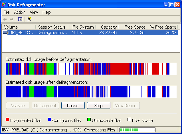
The JVM is a generational, meaning objects are created in an “Eden” space and over time promoted up into the Survivor space and later the Old Generation. This is an attempt to reduce memory fragmentation by keeping objects with a high churn rate limited to a specific memory space. High object churn and fragmentation is problematic because it requires quite a bit of housekeeping to defragment the space. Remember how painful defragmenting a hard drive was?

The JVM has many options for startup settings related to Garbage Collection. First, we’re able to set how much memory the JVM is allowed to use in total. The total space is governed by -Xmx (x for max). We generally set -Xms as well (think ‘s’ for startup) which is how much memory is allocated at startup. For performance reasons, Xmx and Xms should be the same value. If not explicitly set, the Cassandra start script will calculate how much memory to use, with a max of 8GB. This is a safe default that hasn’t changed over the years, but there are many workloads that these settings are not optimal. There’s additional settings that govern the behavior of the collectors, but we will limit the scope of this post to explaining how to correctly size each of the regions, and address the additional parameters in a follow up post.

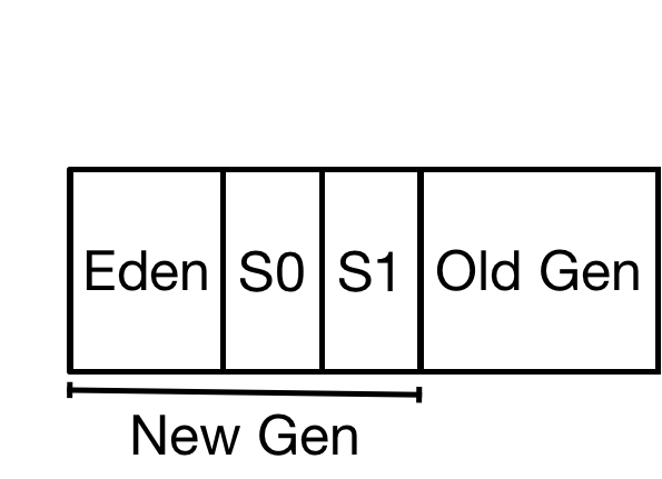
The first two spaces, Eden and survivor, are considered the New Gen, and the sizing is determined by the -Xmn flag. Try to remember n for new. Objects are allocated in the Eden space. Eden is not sized directly, rather it is the remainder of space after we allocate our next region, the survivor spaces.

The survivor space is split into two smaller spaces, referred to S0 and S1. Only one survivor space is active at a given time. We copy objects between the two survivor generations until we eventually promote them to the old generation. The amount of memory in each survivor space is governed by the startup flag -XX:SurvivorRatio. Each survivor space has a 1:SurvivorRatio relationship to the Eden space. If we use the setting -XX:SurvivorRatio=2 with a NewGen of 4GB, Eden will be allocated 2GB of space with each survivor allocated 1GB of space, giving us our 1:2 ratio.

The old generation is where objects eventually land that have survived multiple copies. The idea here is that if they’ve been able to survive this far, they probably will survive a while longer.

Collection and Promotion

Understanding what happens to objects during their lifetime is essential to tuning the JVM optimally. Generally speaking, during each phase the JVM looks at the object graph, determine the objects that are live and which are garbage.

Parallel New

As mentioned above, Eden is where objects are first allocated. This is a fixed size space determined by the -Xmn flag. As objects are allocated in Eden, the space fills up. Once we’ve filled up Eden space, we have our first GC pause. At this time, the JVM stops all threads and inspects the objects in memory. We refer to this as a “stop the world” pause.

We mentioned above only one survivor space is active at any given time. The first thing the JVM does during a ParNew pause is take any objects that are in the current survivor space that are live objects and either copy them to the other survivor space or the old gen, depending on how long they have lived. The number of times is is guided by the XX:MaxTenuringThreshold option, but there is no guarantee that an object has to survive this many times. Any objects that are garbage the JVM does nothing with, they are simply overwritten later. The process of copying objects between generations takes significantly longer than doing nothing, there’s a direct relationship between the number and size of objects copied and how long it takes to copy them. This process all occurs during the stop the world pause. The more we copy, the longer it takes. The bigger the space, the more potential copying we could do. A massive NewGen filled with live objects that need to be promoted would result in massive pauses. On the other hand, a massive new gen filled with garbage that can be disregarded will have very short pauses.

After the surviving objects are copied from one survivor generation to the other, we copy any live objects from the Eden space to the new active survivor space. As with the first phase, copying is slow, cleaning up garbage is fast.

Concurrent Mark and Sweep

In our old generation, we use a different algorithm, Concurrent Mark and Sweep (CMS). The pauses here are shorter, because most of the work is done concurrently with the application. We have two short pauses here, the mark and remark phases. During these pauses we identify the live and dead objects. We’re able to clean up the garbage while the application is running. CMS kicks in when we reach a certain threshold of fullness, specified by the -XX:CMSInitiatingOccupancyFraction parameter. This default is around 92, and somewhat dangerous, we risk memory filling up before CMS can complete. Cassandra sets this to be a bit lower, -XX:CMSInitiatingOccupancyFraction=75 by default is signficantly safer.

Full GC

Full GC happens when we can’t promote objects to the Old Generation. It cleans up all the spaces, freeing up as much space as possible, and does the dreaded defragmention. Full GC pauses are awful, they can lock up the JVM for several minutes, more than enough time for a node to appear as offline. We want to do our best to avoid Full GC pauses. In many cases it’s faster to reboot a node than let it finish a pause lasting several minutes.

Performance Profiles

The key takeaways from the previous section:

• Cleaning up garbage is fast.
• Promoting objects is slow.
• The more promotion, the longer the pause.
• Big spaces are capable of more promotion, and thus, longer pauses.

Figuring out the optimal settings for your Cassandra installation is dependent on the workload. Generally speaking, we can categorize a workload as write heavy, read heavy, or an evenly mixed workload. Almost every cluster we’ve analyzed has fallen into one of the first two workloads, with over 99% of the operations being either reads or writes.

Write Heavy Workloads

Write heavy workloads are the Bread and butter of Cassandra. Writes are optimized by treating Memtables as a write back cache, avoiding random reads and in place updates in favor of bulk writes to memtables and a compaction process (the defining characteristics of an LSM)

During a write heavy workload, there are two primary sources of allocations that we must keep in mind when tuning Garbage Collection: memtables and compaction.

The amount of space used by Memtables is configurable and is a significant source of allocation. Mutations are stored in memtables and flushed to disk as SSTables. If you’re storing large text fields or blobs, you can keep a significant amount of data off heap by enabling the following:

memtable_allocation_type: offheap_objects

Since objects assocated with memtables are being allocated often and kept around for a while, we want to limit the size of our Memtables by explicitly specifying memtable_heap_space_in_mb, otherwise it’s set automatically to 1/4 of the heap. If we limit the space used by Memtables we can safely increase the size of the new gen, which will reduce the frequency of GC pauses.

Compaction can generate a significant amount of garbage, depending on the setting for compaction_throughput_mb_per_sec. Compaction can generate a significant amount of short lived objects. For time series data (the most common write heavy use case), LeveledCompactionStrategy not only generates more I/O and takes up a ton of CPU but also generates significantly more garbage than the more appropriate TimeWindowCompactionStrategy. Alex goes into detail on the behavior of TWCS in this post. Picking the right compaction strategy for the right workload can mean orders of magnitude difference in performance.

Generally speaking, with faster disks and higher compaction throughput, it’s a good idea to increase the size of the new generation to account for faster allocation.

Read Heavy Workloads

Read heavy workloads are a little different. Under a read heavy workload, we have significantly less memory churn related to Memtables. Instead, we have a lot of short lived objects as a result of reads pulling data off disk and creating temporary objects. These objects typically last less than a second, sometimes only a few milliseconds. The faster our disks, the higher the allocation rate.

The trouble with the Cassandra defaults and read heavy workloads is that the new generation is capped at 800MB, and the object allocation rate with fast disks can easily cause objects to be prematurely pushed into the old generation. This is bad because:

• Promotion is slow
• Lots of promotion can easily fill the old gen

With read heavy workloads and fast disks, we need to increase our heap size and new gen or we will suffer incredibly long pauses. A good starting point is to bump up the heap to 12GB and set the size of the new generation to 6GB. This allows us to keep objects associated with reads in the new generation while keeping premature promotion to a minimum. We can also see a significant benefit by increasing XX:MaxTenuringThreshold, which will keep objects in the new gen rather than promoting them. Using larger survivor spaces helps here as well. Starting with -XX:SurvivorRatio=4 instead of the default 8 and XX:MaxTenuringThreshold=6 will keep objects in the new gen a little longer. If your systems have plenty of RAM, 16GB heap with 10GB new gen will decrease the frequency of pauses even more and should keep roughly the same pause times. There’s very little benefit from having a large old generation as we aren’t keeping more long term objects around with the larger heaps.

Final Thoughts

At this point you should have a better understanding of how different workloads behave in the JVM. No matter the workload, the goal is to keep object promotion to a minimum to limit the length of GC pauses. This is one way we keep our important read and write latency metrics low.

This post is by no means an exhaustive list of everything going on inside the JVM, and there’s quite a few opportunities for improvements after this. That said, we’ve seen some really impressive results just from tuning a handful of settings, so this is a great starting point. Significantly decreasing the objects promoted to old gen can reduce GC pauses by an order of magnitude. We’ll be circling back in the future to examine each of the workloads in greater detail.