One of the challenges of running large scale distributed systems is being able to pinpoint problems. It’s all too common to blame a random component (usually a database) whenever there’s a hiccup even when there’s no evidence to support the claim. We’ve already discussed the importance of monitoring tools, graphing and alerting metrics, and using distributed tracing systems like ZipKin to correctly identify the source of a problem in a complex system.

Once you’ve narrowed down the problem to a single system, what do you do? To figure this out, it’s going to depend on the nature of the problem, of course. Some issues are temporary, like a dead disk. Some are related to a human-introduced change, like a deployment or a wrong configuration setting. These have relatively straightforward solutions. Replace the disk, or rollback the deployment.

What about problems that are outside the scope of a simple change? One external factor that we haven’t mentioned so far is growth. Scale can be a difficult problem to understand because reproducing the issue is often nuanced and complex. These challenges are sometimes measured in throughput, (requests per second), size (terabytes), or latency (5ms p99). For instance, if a database server is able to serve every request out of memory, it may get excellent throughput. As the size of the dataset increases, random lookups are more and more likely to go to disk, decreasing throughput. Time Window Compaction Strategy is a great example of a solution to a scale problem that’s hard to understand unless the numbers are there. The pain of compaction isn’t felt until you’re dealing with a large enough volume of data to cause performance problems.

During the times of failure we all too often find ourselves thinking of the machine and its processes as a black box. Billions of instructions executing every second without the ability to peer inside and understand its mysteries.

Fortunately, we’re not completely blind as to what a machine is doing. For years we’ve had tools like debuggers and profilers available to us. Oracle’s JDK offers us Java Flight Recorder, which we can use to analyze running processes locally or in production:

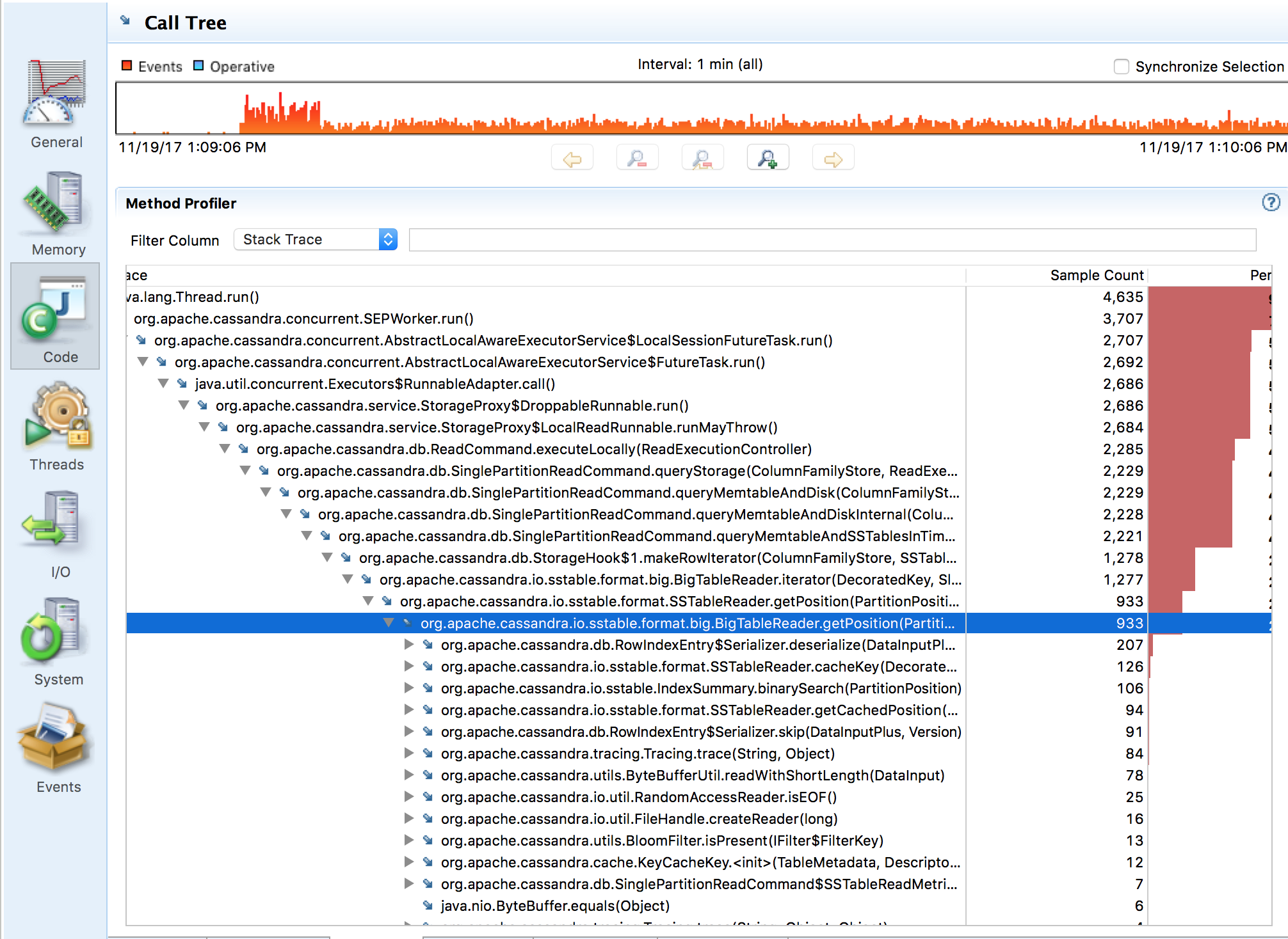
Profiling with flight recorder is straightforward, but interpreting the results takes a little bit of work. Expanding the list of nested tables and looking for obvious issues is a bit more mental work than I’m interested in. It would be a lot easier if we could visualize the information. It requires a commercial license to use in production, and only works with the Oracle JDK.

That brings us back to the subject of this post: a way of generating useful visual information called a flame graph. A flame graph let’s us quickly identify the performance bottlenecks in a system. They were invented by Brendan Gregg. This is also part one of a very long series of performance tuning posts, we will be referring back to it as we dive deeper into the internals of Cassandra.

Swiss Java Knife

The approach we’ll examine in this post is utilizing the Swiss Java Knife, usually referred to as SJK, to capture the data from the JVM and generate the flame graphs. SJK is a fantastic collection of tools. Aside from generating flame graphs, we can inspect garbage collection statistics, watch threads, and do a variety of other diagnostic tasks. It works on Mac, Linux, and both the Oracle JDK and the OpenJDK.

I’ve downloaded the JAR, put it in my $HOME/bin and set up a shell function to call it easily:

sjk () {
	java -jar ~/bin/sjk-plus-0.8.jar "$@"
}

On my laptop I’m running a workload with cassandra-stress. I’ve prepopulated the database, and started the stress workload with the following command:

cassandra-stress read n=1000000

For the first step of our analysis, we need to capture the stack frames of our running Java application using the stcap feature of SJK. To do this, we need to pass in the process id and the file to which we will dump the data. The dumps are written in a binary format that we’ll be able to query later:

sjk stcap -p 92541 -i 10ms -o dump.std

Then we can analyze the data. If all we have is a terminal, we can print out a histogram of the analysis. This can be pretty useful on it’s own if there’s an obvious issue. In this case, we can see that a lot of time is spent in sun.misc.Unsafe.park, meaning threads are just waiting around, parked:

$ sjk ssa -f dump.std --histo
Trc     (%)  Frm  N  Term    (%)  Frame
372447  96%  372447       0   0%  java.lang.Thread.run(Thread.java:745)
309251  80%  309251  309251  80%  sun.misc.Unsafe.park(Native Method)
259376  67%  259376       0   0%  java.util.concurrent.locks.LockSupport.park(LockSupport.java:304)
254388  66%  254388       0   0%  org.apache.cassandra.concurrent.SEPWorker.run(SEPWorker.java:87)
 55709  14%  55709        0   0%  java.util.concurrent.ThreadPoolExecutor$Worker.run(ThreadPoolExecutor.java:617)
 52374  13%  52374        0   0%  org.apache.cassandra.concurrent.NamedThreadFactory$$Lambda$6/1758056825.run(Unknown Source)
 52374  13%  52374        0   0%  org.apache.cassandra.concurrent.NamedThreadFactory.lambda$threadLocalDeallocator$0(NamedThreadFactory.java:81)
 44892  11%  44892        0   0%  io.netty.util.concurrent.DefaultThreadFactory$DefaultRunnableDecorator.run(DefaultThreadFactory.java:138)
 44887  11%  44887        0   0%  java.util.concurrent.ThreadPoolExecutor.runWorker(ThreadPoolExecutor.java:1127)
 42398  11%  42398        0   0%  io.netty.channel.nio.NioEventLoop.run(NioEventLoop.java:409)
 42398  11%  42398        0   0%  io.netty.util.concurrent.SingleThreadEventExecutor$5.run(SingleThreadEventExecutor.java:858)
 42398  11%  42398        0   0%  io.netty.channel.nio.NioEventLoop.select(NioEventLoop.java:753)
 42398  11%  42398        0   0%  sun.nio.ch.KQueueArrayWrapper.poll(KQueueArrayWrapper.java:198)
 42398  11%  42398        0   0%  sun.nio.ch.KQueueSelectorImpl.doSelect(KQueueSelectorImpl.java:117)
 42398  11%  42398    42398  11%  sun.nio.ch.KQueueArrayWrapper.kevent0(Native Method)
 42398  11%  42398        0   0%  sun.nio.ch.SelectorImpl.lockAndDoSelect(SelectorImpl.java:86)
 42398  11%  42398        0   0%  sun.nio.ch.SelectorImpl.select(SelectorImpl.java:97)

Now that we have our stcap dump, we can generate a flame graph with the following command:

sjk ssa --flame -f dump.std > flame-sjk.svg

When you open the SVG in a browser, you should end up with an image which looks something like this:

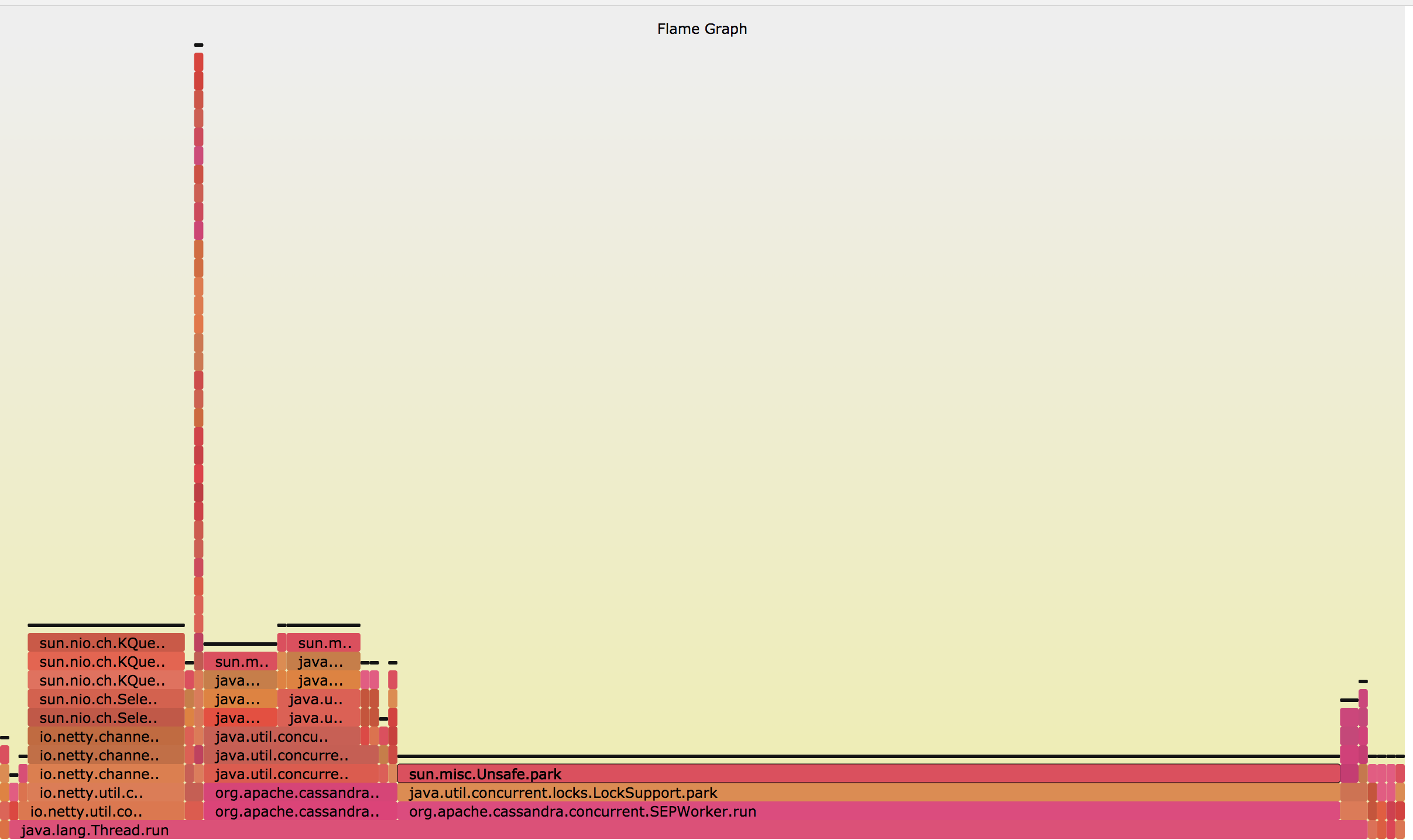
If you open the flame graph on your machine you can mouse over the different sections to see the method call and percentage of time it’s taking. The wider the bar, the more frequent it’s present in the stacks. It’s very easy to glance at the graph to understand where the time is spent in our program.

This is not the only technique for generating flame graphs. Brendan Gregg has a long list of links and references I recommend reading at the bottom of his FlameGraph page. I intend to write a utility to export the SJK format to the format that Brendan uses on his blog as it’s a little nicer to look, has a better mouseover, supports drill down, and has a search. They also support differential flame graphs, which are nice if you’re doing performance comparisons across different builds.

I hope you’ve enjoyed this post on visualizing Cassandra’s performance using FlameGraphs. We’ve used this tool several times with the teams we’ve worked with to tune Cassandra’s configurations and optimize performance. In the next post in this series we’ll be examining how to tune garbage collection parameters to maximize throughput while keeping latency to a minimum.