Benchmarking schemas and configuration changes using the cassandra-stress tool, before pushing such changes out to production is one of the things every Cassandra developer should know and regularly practice.

But wouldn’t it be nice if you could graph the output of it?

Graph it!

The cassandra-stress tool, originally known as just stress, has been around a long time going all the way back to Cassandra-0.5. It has evolved over the years and today using it in its simplest form is along the lines of…

cassandra-stress write n=10000 -rate threads=10
cassandra-stress mixed n=10000 -rate threads=10

When running cassandra-stress you need to run the benchmark first in write mode. After that then you are free to run in read or mixed mode. And the output of it is rather old-school looking like…

Created keyspaces. Sleeping 1s for propagation.
Sleeping 2s...
Warming up WRITE with 50000 iterations...
INFO  21:41:38 New Cassandra host localhost/127.0.0.1:9042 added
Connected to cluster: Test Cluster
Datatacenter: datacenter1; Host: localhost/127.0.0.1; Rack: rack1
Running WRITE with 10 threads for 10000 iteration
type,      total ops,    op/s,    pk/s,   row/s,    mean,     med,     .95,     .99,    .999,     max,   time,   stderr, errors,  gc: #,  max ms,  sum ms,  sdv ms,      mb
total,         10000,   16386,   16386,   16386,     0.6,     0.4,     1.3,     3.4,    23.4,    25.7,    0.6,  0.00000,      0,      1,      17,      17,       0,     308


Results:
op rate                   : 16386 [WRITE:16386]
partition rate            : 16386 [WRITE:16386]
row rate                  : 16386 [WRITE:16386]
latency mean              : 0.6 [WRITE:0.6]
latency median            : 0.4 [WRITE:0.4]
latency 95th percentile   : 1.3 [WRITE:1.3]
latency 99th percentile   : 3.4 [WRITE:3.4]
latency 99.9th percentile : 23.4 [WRITE:23.4]
latency max               : 25.7 [WRITE:25.7]
Total partitions          : 10000 [WRITE:10000]
Total errors              : 0 [WRITE:0]
total gc count            : 1
total gc mb               : 308
total gc time (s)         : 0
avg gc time(ms)           : 17
stdev gc time(ms)         : 0
Total operation time      : 00:00:00
END

There’s a lot of useful information here especially in the summary. But making effecient use of that middle section is cumbersome especially when the n= option becomes a much larger and more realistic stress number. Comparing consistency of latency numbers or investigating how 99th percentile latencies come about involves a bit of digging.

The lack of graphing ability to cassandra-stress was raised over a year ago by Benedict, as DataStax’s big brother to cassandra-stress: cstar_perf; has such graphing ability already and to which graphs you’ve probably seen before attached to various Cassandra jira issues and Planet Cassandra blog posts. Benedict had in fact gone further pointing out the need for even more graphing than want cstart_perf does today, which seems to be in the works now under CASSANDRA-9870.

Once the patch from CASSANDRA-7918 hits trunk, or if you’re willing to checkout engima curry’s cassandra fork and build it yourself, to generate pretty graphs with cassandra-stress is as simple as…

cassandra-stress write n=100000 -rate threads=10 -graph file=example-benchmark.html title=example revision=benchmark-0

cassandra-stress mixed n=100000 -rate threads=10 -graph file=example-benchmark.html title=example revision=benchmark-0

Now in the current directory you’ll find an example-benchmark.html file. Opening this shows the pretty graphs with both write and read benchmarks for the “benchmark-0” revision. In the following graphs the benchmarch was against a specific version of C* and so the revision is named just “cassandra-A” and here the number of requests was increased to ten million.

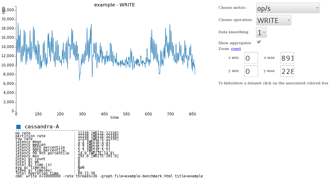
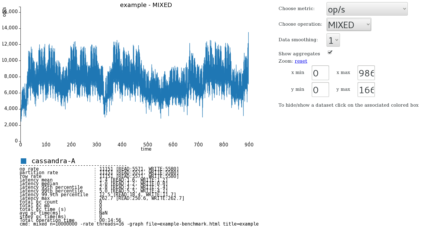
The nice thing about this html file is that it’s completely standalone so sharing it and posting it to jira issues is a simple practical thing to do. On top of that you just keep running further benchmarks with new revision names and they’ll get added to the existing graph. For example let’s run a new benchmark revision

cassandra-stress write n=100000 -rate threads=10 -graph file=example-benchmark.html title=example revision=benchmark-1

cassandra-stress mixed n=100000 -rate threads=10 -graph file=example-benchmark.html title=example revision=benchmark-1

Refresh the graph and you see the comparison clearly between the two revisions now. In the next graphs I added three new revisions “cassandra-B”, “cassandra-C”, and “cassandra-D”. Take these graphs with a pinch of salt, they were run on my dual-core laptop, but they show just how just valuable a little visualisation can be.

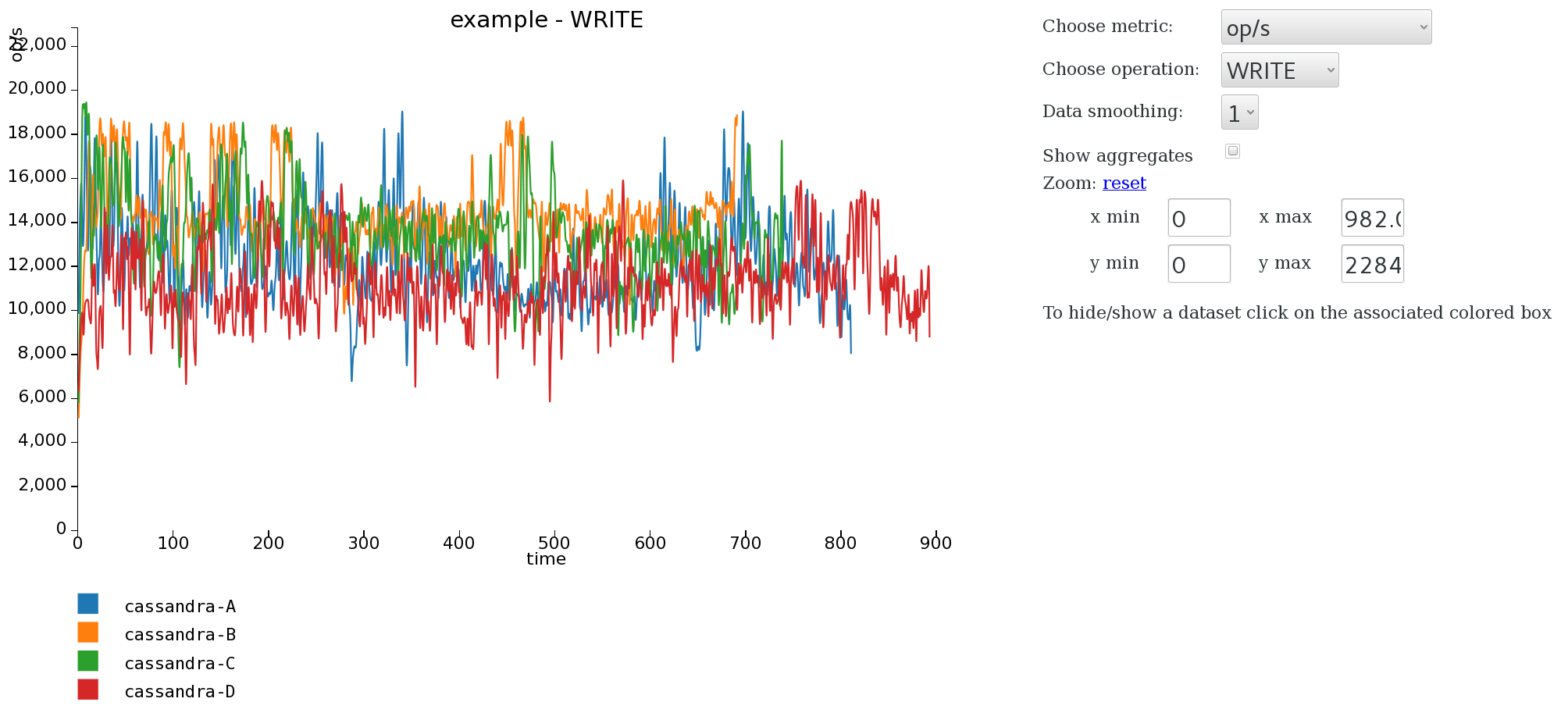
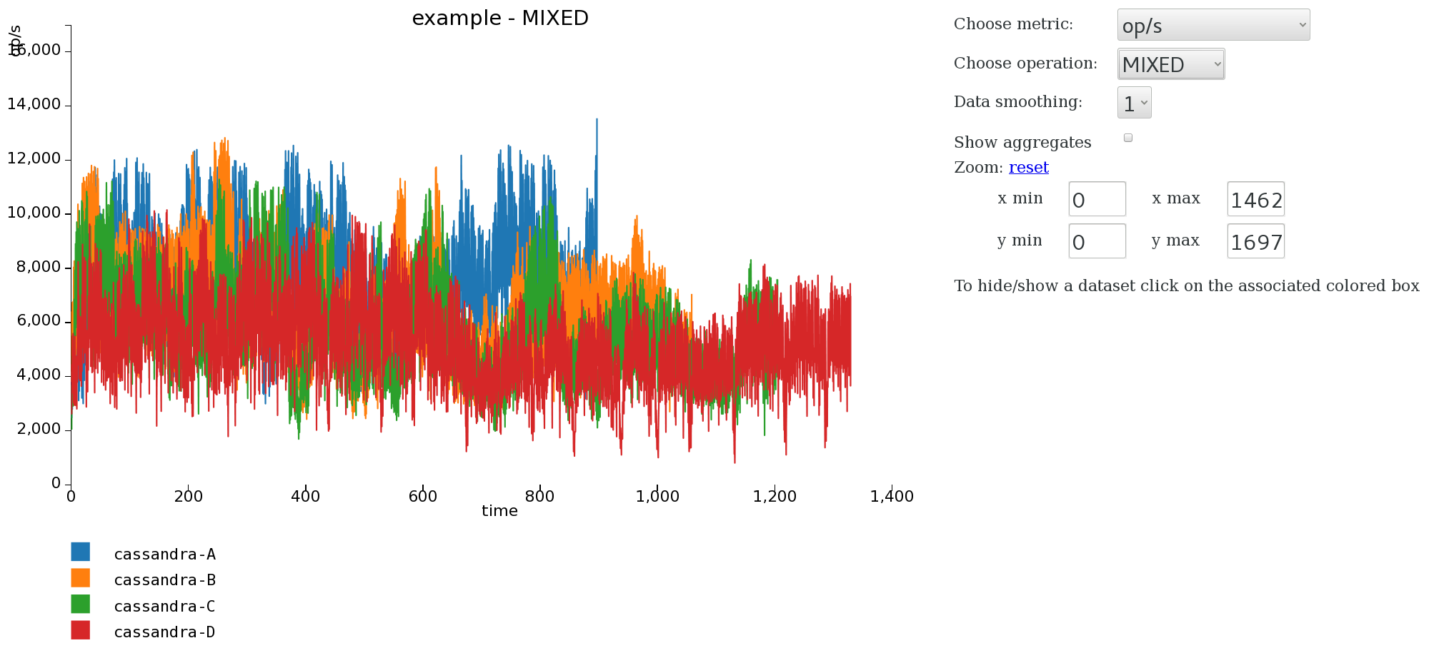
So simple.