![]()
Anthony Grasso
The Impacts of Changing the Number of VNodes in Apache Cassandra
Apache Cassandra’s default value for num_tokens is about to change in 4.0! This might seem like a small edit note in the CHANGES.txt, however such a change can have a profound effect on day-to-day operations of the cluster. In this post we will examine how changing the value for num_tokens impacts the cluster and its behaviour.
There are many knobs and levers that can be modified in Apache Cassandra to tune its behaviour. The num_tokens setting is one of those. Like many settings it lives in the cassandra.yaml file and has a defined default value. That’s where it stops being like many of Cassandra’s settings. You see, most of Cassandra’s settings will only affect a single aspect of the cluster. However, when changing the value of num_tokens there is an array of behaviours that are altered. The Apache Cassandra project has committed and resolved CASSANDRA-13701 which changed the default value for num_tokens from 256 to 16. This change is significant, and to understand the consequences we first need to understand the role that num_tokens play in the cluster.
Never try this on production
Before we dive into any details it is worth noting that the num_tokens setting on a node should never ever be changed once it has joined the cluster. For one thing the node will fail on a restart. The value of this setting should be the same for every node in a datacenter. Historically, different values were expected for heterogeneous clusters. While it’s rare to see, nor would we recommend, you can still in theory double the num_tokens on nodes that are twice as big in terms of hardware specifications. Furthermore, it is common to see the nodes in a datacenter have a value for num_tokens that differs to nodes in another datacenter. This is partly how changing the value of this setting on a live cluster can be safely done with zero downtime. It is out of scope for this blog post, but details can be found in migration to a new datacenter.
The Basics
The num_tokens setting influences the way Cassandra allocates data amongst the nodes, how that data is retrieved, and how that data is moved between nodes.
Under the hood Cassandra uses a partitioner to decide where data is stored in the cluster. The partitioner is a consistent hashing algorithm that maps a partition key (first part of the primary key) to a token. The token dictates which nodes will contain the data associated with the partition key. Each node in the cluster is assigned one or more unique token values from a token ring. This is just a fancy way of saying each node is assigned a number from a circular number range. That is, “the number” being the token hash, and “a circular number range” being the token ring. The token ring is circular because the next value after the maximum token value is the minimum token value.
An assigned token defines the range of tokens in the token ring the node is responsible for. This is commonly known as a “token range”. The “token range” a node is responsible for is bounded by its assigned token, and the next smallest token value going backwards in the ring. The assigned token is included in the range, and the smallest token value going backwards is excluded from the range. The smallest token value going backwards typically resides on the previous neighbouring node. Having a circular token ring means that the range of tokens a node is responsible for, could include both the minimum and maximum tokens in the ring. In at least one case the smallest token value going backwards will wrap back past the maximum token value in the ring.
For example, in the following Token Ring Assignment diagram we have a token ring with a range of hashes from 0 to 99. Token 10 is allocated to Node 1. The node before Node 1 in the cluster is Node 5. Node 5 is allocated token 90. Therefore, the range of tokens that Node 1 is responsible for is between 91 and 10. In this particular case, the token range wraps around past the maximum token in the ring.
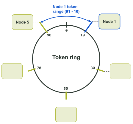
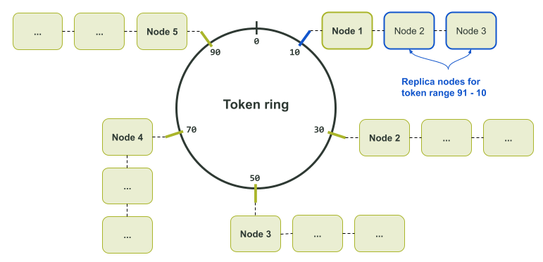
Note that the above diagram is for only a single data replica. This is because only a single node is assigned to each token in the token ring. If multiple replicas of the data exists, a node’s neighbours become replicas for the token as well. This is illustrated in the Token Ring Assignment diagram below.
The reason the partitioner is defined as a consistent hashing algorithm is because it is just that; no matter how many times you feed in a specific input, it will always generate the same output value. It ensures that every node, coordinator, or otherwise, will always calculate the same token for a given partition key. The calculated token can then be used to reliably pinpoint the nodes with the sought after data.
Consequently, the minimum and maximum numbers for the token ring are defined by the partitioner. The default Murur3Partitioner based on the Murmur hash has for example, a minimum and maximum range of -2^63 to +2^63 - 1. The legacy RandomPartitioner (based on the MD5 hash) on the other hand has a range of 0 to 2^127 - 1. A critical side effect of this system is that once a partitioner for a cluster is picked, it can never be changed. Changing to a different partitioner requires the creation of a new cluster with the desired partitioner and then reloading the data into the new cluster.
Further information on consistent hashing functionality can be found in the Apache Cassandra documentation.
Back in the day…
Back in the pre-1.2 era, nodes could only be manually assigned a single token. This was done and can still be done today using the initial_token setting in the cassandra.yaml file. The default partitioner at that point was the RandomPartitioner. Despite token assignment being manual, the partitioner made the process of calculating the assigned tokens fairly straightforward when setting up a cluster from scratch. For example, if you had a three node cluster you would divide 2^127 - 1 by 3 and the quotient would give you the correct increment amount for each token value. Your first node would have an initial_token of 0, your next node would have an initial_token of (2^127 - 1) / 3, and your third node would have an initial_token of (2^127 - 1) / 3 * 2. Thus, each node will have the same sized token ranges.
Dividing the token ranges up evenly makes it less likely individual nodes are overloaded (assuming identical hardware for the nodes, and an even distribution of data across the cluster). Uneven token distribution can result in what is termed “hot spots”. This is where a node is under pressure as it is servicing more requests or carrying more data than other nodes.
Even though setting up a single token cluster can be a very manual process, their deployment is still common. Especially for very large Cassandra clusters where the node count typically exceeds 1,000 nodes. One of the advantages of this type of deployment, is you can ensure that the token distribution is even.
Although setting up a single token cluster from scratch can result in an even load distribution, growing the cluster is far less straight forward. If you insert a single node into your three node cluster, the result is that two out of the four nodes will have a smaller token range than the other two nodes. To fix this problem and re-balance, you then have to run nodetool move to relocate tokens to other nodes. This is a tedious and expensive task though, involving a lot of streaming around the whole cluster. The alternative is to double the size of your cluster each time you expand it. However, this usually means using more hardware than you need. Much like having an immaculate backyard garden, maintaining an even token range per node in a single token cluster requires time, care, and attention, or alternatively, a good deal of clever automation.
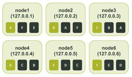
Scaling in a single token world is only half the challenge. Certain failure scenarios heavily reduce time to recovery. Let’s say for example you had a six node cluster with three replicas of the data in a single datacenter (Replication Factor = 3). Replicas might reside on Node 1 and Node 4, Node 2 and Node 5, and lastly on Node 3 and Node 6. In this scenario each node is responsible for a sixth of each of the three replicas.
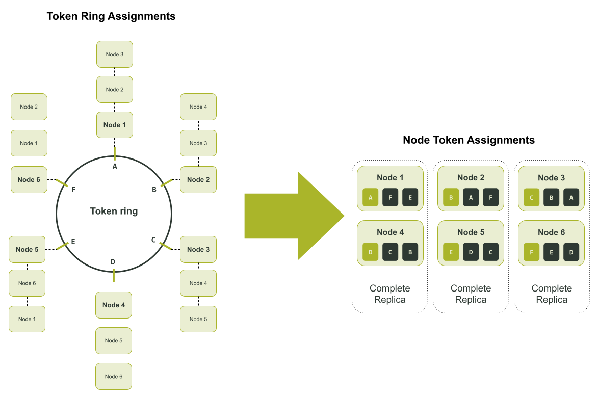
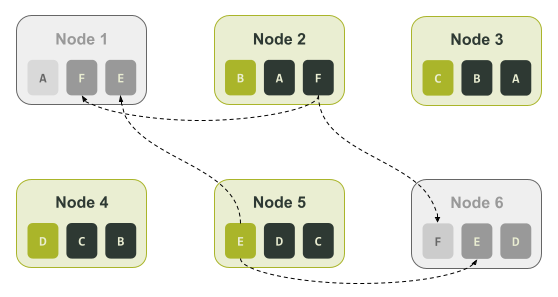
In the above diagram, the tokens in the token ring are assigned an alpha character. This is to make tracking the token assignment to each node easier to follow. If the cluster had an outage where Node 1 and Node 6 are unavailable, you could only use Nodes 2 and 5 to recover the unique sixth of the data they each have. That is, only Node 2 could be used to recover the data associated with token range ‘F’, and similarly only Node 5 could be used to recover the data associated with token range ‘E’. This is illustrated in the diagram below.
vnodes to the rescue
To solve the shortcomings of a single token assignment, Cassandra version 1.2 was enhanced to allow a node to be assigned multiple tokens. That is a node could be responsible for multiple token ranges. This Cassandra feature is known as “virtual node” or vnodes for short. The vnodes feature was introduced via CASSANDRA-4119. As per the ticket description, the goals of vnodes were:
- Reduced operations complexity for scaling up/down.
- Reduced rebuild time in event of failure.
- Evenly distributed load impact in the event of failure.
- Evenly distributed impact of streaming operations.
- More viable support for heterogeneity of hardware.
The introduction of this feature gave birth to the num_tokens setting in the cassandra.yaml file. The setting defined the number of vnodes (token ranges) a node was responsible for. By increasing the number of vnodes per node, the token ranges become smaller. This is because the token ring has a finite number of tokens. The more ranges it is divided up into the smaller each range is.
To maintain backwards compatibility with older 1.x series clusters, the num_tokens defaulted to a value of 1. Moreover, the setting was effectively disabled on a vanilla installation. Specifically, the value in the cassandra.yaml file was commented out. The commented line and previous development commits did give a glimpse into the future of where the feature was headed though.
As foretold by the cassandra.yaml file, and the git commit history, when Cassandra version 2.0 was released out the vnodes feature was enabled by default. The num_tokens line was no longer commented out, so its effective default value on a vanilla installation was 256. Thus ushering in a new era of clusters that had relatively even token distributions, and were simple to grow.
With nodes consisting of 256 vnodes and the accompanying additional features, expanding the cluster was a dream. You could insert one new node into your cluster and Cassandra would calculate and assign the tokens automatically! The token values were randomly calculated, and so over time as you added more nodes, the cluster would converge on being in a balanced state. This engineering wizardry put an end to spending hours doing calculations and nodetool move operations to grow a cluster. The option was still there though. If you had a very large cluster or another requirement, you could still use the initial_token setting which was commented out in Cassandra version 2.0. In this case, the value for the num_tokens still had to be set to the number of tokens manually defined in the initial_token setting.
Remember to read the fine print
This gave us a feature that was like a personal devops assistant; you handed them a node, told them to insert it, and then after some time it had tokens allocated and was part of the cluster. However, in a similar vein, there is a price to pay for the convenience…
While we get a more even token distribution when using 256 vnodes, the problem is that availability degrades earlier. Ironically, the more we break the token ranges up the more quickly we can get data unavailability. Then there is the issue of unbalanced token ranges when using a small number of vnodes. By small, I mean values less than 32. Cassandra’s random token allocation is hopeless when it comes to small vnode values. This is because there are insufficient tokens to balance out the wildly different token range sizes that are generated.
Pics or it didn’t happen
It is very easy to demonstrate the availability and token range imbalance issues, using a test cluster. We can set up a single token range cluster with six nodes using ccm. After calculating the tokens, configuring and starting our test cluster, it looked like this.
$ ccm node1 nodetool status

Datacenter: datacenter1
=======================
Status=Up/Down
|/ State=Normal/Leaving/Joining/Moving
--  Address    Load       Tokens       Owns (effective)  Host ID                               Rack
UN  127.0.0.1  71.17 KiB  1            33.3%             8d483ae7-e7fa-4c06-9c68-22e71b78e91f  rack1
UN  127.0.0.2  65.99 KiB  1            33.3%             cc15803b-2b93-40f7-825f-4e7bdda327f8  rack1
UN  127.0.0.3  85.3 KiB   1            33.3%             d2dd4acb-b765-4b9e-a5ac-a49ec155f666  rack1
UN  127.0.0.4  104.58 KiB  1            33.3%             ad11be76-b65a-486a-8b78-ccf911db4aeb  rack1
UN  127.0.0.5  71.19 KiB  1            33.3%             76234ece-bf24-426a-8def-355239e8f17b  rack1
UN  127.0.0.6  30.45 KiB  1            33.3%             cca81c64-d3b9-47b8-ba03-46356133401b  rack1
We can then create a test keyspace and populated it using cqlsh.
$ ccm node1 cqlsh
Connected to SINGLETOKEN at 127.0.0.1:9042.
[cqlsh 5.0.1 | Cassandra 3.11.9 | CQL spec 3.4.4 | Native protocol v4]
Use HELP for help.
cqlsh> CREATE KEYSPACE test_keyspace WITH REPLICATION = { 'class' : 'NetworkTopologyStrategy', 'datacenter1' : 3 };
cqlsh> CREATE TABLE test_keyspace.test_table (
...   id int,
...   value text,
...   PRIMARY KEY (id));
cqlsh> CONSISTENCY LOCAL_QUORUM;
Consistency level set to LOCAL_QUORUM.
cqlsh> INSERT INTO test_keyspace.test_table (id, value) VALUES (1, 'foo');
cqlsh> INSERT INTO test_keyspace.test_table (id, value) VALUES (2, 'bar');
cqlsh> INSERT INTO test_keyspace.test_table (id, value) VALUES (3, 'net');
cqlsh> INSERT INTO test_keyspace.test_table (id, value) VALUES (4, 'moo');
cqlsh> INSERT INTO test_keyspace.test_table (id, value) VALUES (5, 'car');
cqlsh> INSERT INTO test_keyspace.test_table (id, value) VALUES (6, 'set');
To confirm that the cluster is perfectly balanced, we can check the token ring.
$ ccm node1 nodetool ring test_keyspace


Datacenter: datacenter1
==========
Address    Rack   Status  State   Load        Owns     Token
                                                       6148914691236517202
127.0.0.1  rack1  Up      Normal  125.64 KiB  50.00%   -9223372036854775808
127.0.0.2  rack1  Up      Normal  125.31 KiB  50.00%   -6148914691236517206
127.0.0.3  rack1  Up      Normal  124.1 KiB   50.00%   -3074457345618258604
127.0.0.4  rack1  Up      Normal  104.01 KiB  50.00%   -2
127.0.0.5  rack1  Up      Normal  126.05 KiB  50.00%   3074457345618258600
127.0.0.6  rack1  Up      Normal  120.76 KiB  50.00%   6148914691236517202
We can see in the “Owns” column all nodes have 50% ownership of the data. To make the example easier to follow we can manually add a letter representation next to each token number. So the token ranges could be represented in the following way:
$ ccm node1 nodetool ring test_keyspace


Datacenter: datacenter1
==========
Address    Rack   Status  State   Load        Owns     Token                 Token Letter
                                                       6148914691236517202   F
127.0.0.1  rack1  Up      Normal  125.64 KiB  50.00%   -9223372036854775808  A
127.0.0.2  rack1  Up      Normal  125.31 KiB  50.00%   -6148914691236517206  B
127.0.0.3  rack1  Up      Normal  124.1 KiB   50.00%   -3074457345618258604  C
127.0.0.4  rack1  Up      Normal  104.01 KiB  50.00%   -2                    D
127.0.0.5  rack1  Up      Normal  126.05 KiB  50.00%   3074457345618258600   E
127.0.0.6  rack1  Up      Normal  120.76 KiB  50.00%   6148914691236517202   F
We can then capture the output of ccm node1 nodetool describering test_keyspace and change the token numbers to the corresponding letters in the above token ring output.
$ ccm node1 nodetool describering test_keyspace

Schema Version:6256fe3f-a41e-34ac-ad76-82dba04d92c3
TokenRange:
  TokenRange(start_token:A, end_token:B, endpoints:[127.0.0.2, 127.0.0.3, 127.0.0.4], rpc_endpoints:[127.0.0.2, 127.0.0.3, 127.0.0.4], endpoint_details:[EndpointDetails(host:127.0.0.2, datacenter:datacenter1, rack:rack1), EndpointDetails(host:127.0.0.3, datacenter:datacenter1, rack:rack1), EndpointDetails(host:127.0.0.4, datacenter:datacenter1, rack:rack1)])
  TokenRange(start_token:C, end_token:D, endpoints:[127.0.0.4, 127.0.0.5, 127.0.0.6], rpc_endpoints:[127.0.0.4, 127.0.0.5, 127.0.0.6], endpoint_details:[EndpointDetails(host:127.0.0.4, datacenter:datacenter1, rack:rack1), EndpointDetails(host:127.0.0.5, datacenter:datacenter1, rack:rack1), EndpointDetails(host:127.0.0.6, datacenter:datacenter1, rack:rack1)])
  TokenRange(start_token:B, end_token:C, endpoints:[127.0.0.3, 127.0.0.4, 127.0.0.5], rpc_endpoints:[127.0.0.3, 127.0.0.4, 127.0.0.5], endpoint_details:[EndpointDetails(host:127.0.0.3, datacenter:datacenter1, rack:rack1), EndpointDetails(host:127.0.0.4, datacenter:datacenter1, rack:rack1), EndpointDetails(host:127.0.0.5, datacenter:datacenter1, rack:rack1)])
  TokenRange(start_token:D, end_token:E, endpoints:[127.0.0.5, 127.0.0.6, 127.0.0.1], rpc_endpoints:[127.0.0.5, 127.0.0.6, 127.0.0.1], endpoint_details:[EndpointDetails(host:127.0.0.5, datacenter:datacenter1, rack:rack1), EndpointDetails(host:127.0.0.6, datacenter:datacenter1, rack:rack1), EndpointDetails(host:127.0.0.1, datacenter:datacenter1, rack:rack1)])
  TokenRange(start_token:F, end_token:A, endpoints:[127.0.0.1, 127.0.0.2, 127.0.0.3], rpc_endpoints:[127.0.0.1, 127.0.0.2, 127.0.0.3], endpoint_details:[EndpointDetails(host:127.0.0.1, datacenter:datacenter1, rack:rack1), EndpointDetails(host:127.0.0.2, datacenter:datacenter1, rack:rack1), EndpointDetails(host:127.0.0.3, datacenter:datacenter1, rack:rack1)])
  TokenRange(start_token:E, end_token:F, endpoints:[127.0.0.6, 127.0.0.1, 127.0.0.2], rpc_endpoints:[127.0.0.6, 127.0.0.1, 127.0.0.2], endpoint_details:[EndpointDetails(host:127.0.0.6, datacenter:datacenter1, rack:rack1), EndpointDetails(host:127.0.0.1, datacenter:datacenter1, rack:rack1), EndpointDetails(host:127.0.0.2, datacenter:datacenter1, rack:rack1)])
Using the above output, specifically the end_token, we can determine all the token ranges assigned to each node. As mentioned earlier, the token range is defined by the values after the previous token (start_token) up to and including the assigned token (end_token). The token ranges assigned to each node looked like this:
In this setup, if node3 and node6 were unavailable, we would lose an entire replica. Even if the application is using a Consistency Level of LOCAL_QUORUM, all the data is still available. We still have two other replicas across the other four nodes.
Now let’s consider the case where our cluster is using vnodes. For example purposes we can set num_tokens to 3. It will give us a smaller number of tokens making for an easier to follow example. After configuring and starting the nodes in ccm, our test cluster initially looked like this.
For the majority of production deployments where the cluster size is less than 500 nodes, it is recommended that you use a larger value for `num_tokens`. Further information can be found in the Apache Cassandra Production Recommendations.
$ ccm node1 nodetool status

Datacenter: datacenter1
=======================
Status=Up/Down
|/ State=Normal/Leaving/Joining/Moving
--  Address    Load       Tokens  Owns (effective)  Host ID                               Rack
UN  127.0.0.1  71.21 KiB  3       46.2%             7d30cbd4-8356-4189-8c94-0abe8e4d4d73  rack1
UN  127.0.0.2  66.04 KiB  3       37.5%             16bb0b37-2260-440c-ae2a-08cbf9192f85  rack1
UN  127.0.0.3  90.48 KiB  3       28.9%             dc8c9dfd-cf5b-470c-836d-8391941a5a7e  rack1
UN  127.0.0.4  104.64 KiB  3      20.7%             3eecfe2f-65c4-4f41-bbe4-4236bcdf5bd2  rack1
UN  127.0.0.5  66.09 KiB  3       36.1%             4d5adf9f-fe0d-49a0-8ab3-e1f5f9f8e0a2  rack1
UN  127.0.0.6  71.23 KiB  3       30.6%             b41496e6-f391-471c-b3c4-6f56ed4442d6  rack1
Right off the blocks we can see signs that the cluster might be unbalanced. Similar to what we did with the single node cluster, here we create the test keyspace and populate it using cqlsh. We then grab a read out of the token ring to see what that looks like. Once again, to make the example easier to follow we manually add a letter representation next to each token number.
$ ccm node1 nodetool ring test_keyspace

Datacenter: datacenter1
==========
Address    Rack   Status  State   Load        Owns    Token                 Token Letter
                                                      8828652533728408318   R
127.0.0.5  rack1  Up      Normal  121.09 KiB  41.44%  -7586808982694641609  A
127.0.0.1  rack1  Up      Normal  126.49 KiB  64.03%  -6737339388913371534  B
127.0.0.2  rack1  Up      Normal  126.04 KiB  66.60%  -5657740186656828604  C
127.0.0.3  rack1  Up      Normal  135.71 KiB  39.89%  -3714593062517416200  D
127.0.0.6  rack1  Up      Normal  126.58 KiB  40.07%  -2697218374613409116  E
127.0.0.1  rack1  Up      Normal  126.49 KiB  64.03%  -1044956249817882006  F
127.0.0.2  rack1  Up      Normal  126.04 KiB  66.60%  -877178609551551982   G
127.0.0.4  rack1  Up      Normal  110.22 KiB  47.96%  -852432543207202252   H
127.0.0.5  rack1  Up      Normal  121.09 KiB  41.44%  117262867395611452    I
127.0.0.6  rack1  Up      Normal  126.58 KiB  40.07%  762725591397791743    J
127.0.0.3  rack1  Up      Normal  135.71 KiB  39.89%  1416289897444876127   K
127.0.0.1  rack1  Up      Normal  126.49 KiB  64.03%  3730403440915368492   L
127.0.0.4  rack1  Up      Normal  110.22 KiB  47.96%  4190414744358754863   M
127.0.0.2  rack1  Up      Normal  126.04 KiB  66.60%  6904945895761639194   N
127.0.0.5  rack1  Up      Normal  121.09 KiB  41.44%  7117770953638238964   O
127.0.0.4  rack1  Up      Normal  110.22 KiB  47.96%  7764578023697676989   P
127.0.0.3  rack1  Up      Normal  135.71 KiB  39.89%  8123167640761197831   Q
127.0.0.6  rack1  Up      Normal  126.58 KiB  40.07%  8828652533728408318   R
As we can see from the “Owns” column above, there are some large token range ownership imbalances. The smallest token range ownership is by node 127.0.0.3 at 39.89%. The largest token range ownership is by node 127.0.0.2 at 66.6%. This is about 26% difference!
Once again, we capture the output of ccm node1 nodetool describering test_keyspace and change the token numbers to the corresponding letters in the above token ring.
$ ccm node1 nodetool describering test_keyspace

Schema Version:4b2dc440-2e7c-33a4-aac6-ffea86cb0e21
TokenRange:
    TokenRange(start_token:J, end_token:K, endpoints:[127.0.0.3, 127.0.0.1, 127.0.0.4], rpc_endpoints:[127.0.0.3, 127.0.0.1, 127.0.0.4], endpoint_details:[EndpointDetails(host:127.0.0.3, datacenter:datacenter1, rack:rack1), EndpointDetails(host:127.0.0.1, datacenter:datacenter1, rack:rack1), EndpointDetails(host:127.0.0.4, datacenter:datacenter1, rack:rack1)])
    TokenRange(start_token:K, end_token:L, endpoints:[127.0.0.1, 127.0.0.4, 127.0.0.2], rpc_endpoints:[127.0.0.1, 127.0.0.4, 127.0.0.2], endpoint_details:[EndpointDetails(host:127.0.0.1, datacenter:datacenter1, rack:rack1), EndpointDetails(host:127.0.0.4, datacenter:datacenter1, rack:rack1), EndpointDetails(host:127.0.0.2, datacenter:datacenter1, rack:rack1)])
    TokenRange(start_token:E, end_token:F, endpoints:[127.0.0.1, 127.0.0.2, 127.0.0.4], rpc_endpoints:[127.0.0.1, 127.0.0.2, 127.0.0.4], endpoint_details:[EndpointDetails(host:127.0.0.1, datacenter:datacenter1, rack:rack1), EndpointDetails(host:127.0.0.2, datacenter:datacenter1, rack:rack1), EndpointDetails(host:127.0.0.4, datacenter:datacenter1, rack:rack1)])
    TokenRange(start_token:D, end_token:E, endpoints:[127.0.0.6, 127.0.0.1, 127.0.0.2], rpc_endpoints:[127.0.0.6, 127.0.0.1, 127.0.0.2], endpoint_details:[EndpointDetails(host:127.0.0.6, datacenter:datacenter1, rack:rack1), EndpointDetails(host:127.0.0.1, datacenter:datacenter1, rack:rack1), EndpointDetails(host:127.0.0.2, datacenter:datacenter1, rack:rack1)])
    TokenRange(start_token:I, end_token:J, endpoints:[127.0.0.6, 127.0.0.3, 127.0.0.1], rpc_endpoints:[127.0.0.6, 127.0.0.3, 127.0.0.1], endpoint_details:[EndpointDetails(host:127.0.0.6, datacenter:datacenter1, rack:rack1), EndpointDetails(host:127.0.0.3, datacenter:datacenter1, rack:rack1), EndpointDetails(host:127.0.0.1, datacenter:datacenter1, rack:rack1)])
    TokenRange(start_token:A, end_token:B, endpoints:[127.0.0.1, 127.0.0.2, 127.0.0.3], rpc_endpoints:[127.0.0.1, 127.0.0.2, 127.0.0.3], endpoint_details:[EndpointDetails(host:127.0.0.1, datacenter:datacenter1, rack:rack1), EndpointDetails(host:127.0.0.2, datacenter:datacenter1, rack:rack1), EndpointDetails(host:127.0.0.3, datacenter:datacenter1, rack:rack1)])
    TokenRange(start_token:R, end_token:A, endpoints:[127.0.0.5, 127.0.0.1, 127.0.0.2], rpc_endpoints:[127.0.0.5, 127.0.0.1, 127.0.0.2], endpoint_details:[EndpointDetails(host:127.0.0.5, datacenter:datacenter1, rack:rack1), EndpointDetails(host:127.0.0.1, datacenter:datacenter1, rack:rack1), EndpointDetails(host:127.0.0.2, datacenter:datacenter1, rack:rack1)])
    TokenRange(start_token:M, end_token:N, endpoints:[127.0.0.2, 127.0.0.5, 127.0.0.4], rpc_endpoints:[127.0.0.2, 127.0.0.5, 127.0.0.4], endpoint_details:[EndpointDetails(host:127.0.0.2, datacenter:datacenter1, rack:rack1), EndpointDetails(host:127.0.0.5, datacenter:datacenter1, rack:rack1), EndpointDetails(host:127.0.0.4, datacenter:datacenter1, rack:rack1)])
    TokenRange(start_token:H, end_token:I, endpoints:[127.0.0.5, 127.0.0.6, 127.0.0.3], rpc_endpoints:[127.0.0.5, 127.0.0.6, 127.0.0.3], endpoint_details:[EndpointDetails(host:127.0.0.5, datacenter:datacenter1, rack:rack1), EndpointDetails(host:127.0.0.6, datacenter:datacenter1, rack:rack1), EndpointDetails(host:127.0.0.3, datacenter:datacenter1, rack:rack1)])
    TokenRange(start_token:L, end_token:M, endpoints:[127.0.0.4, 127.0.0.2, 127.0.0.5], rpc_endpoints:[127.0.0.4, 127.0.0.2, 127.0.0.5], endpoint_details:[EndpointDetails(host:127.0.0.4, datacenter:datacenter1, rack:rack1), EndpointDetails(host:127.0.0.2, datacenter:datacenter1, rack:rack1), EndpointDetails(host:127.0.0.5, datacenter:datacenter1, rack:rack1)])
    TokenRange(start_token:N, end_token:O, endpoints:[127.0.0.5, 127.0.0.4, 127.0.0.3], rpc_endpoints:[127.0.0.5, 127.0.0.4, 127.0.0.3], endpoint_details:[EndpointDetails(host:127.0.0.5, datacenter:datacenter1, rack:rack1), EndpointDetails(host:127.0.0.4, datacenter:datacenter1, rack:rack1), EndpointDetails(host:127.0.0.3, datacenter:datacenter1, rack:rack1)])
    TokenRange(start_token:P, end_token:Q, endpoints:[127.0.0.3, 127.0.0.6, 127.0.0.5], rpc_endpoints:[127.0.0.3, 127.0.0.6, 127.0.0.5], endpoint_details:[EndpointDetails(host:127.0.0.3, datacenter:datacenter1, rack:rack1), EndpointDetails(host:127.0.0.6, datacenter:datacenter1, rack:rack1), EndpointDetails(host:127.0.0.5, datacenter:datacenter1, rack:rack1)])
    TokenRange(start_token:Q, end_token:R, endpoints:[127.0.0.6, 127.0.0.5, 127.0.0.1], rpc_endpoints:[127.0.0.6, 127.0.0.5, 127.0.0.1], endpoint_details:[EndpointDetails(host:127.0.0.6, datacenter:datacenter1, rack:rack1), EndpointDetails(host:127.0.0.5, datacenter:datacenter1, rack:rack1), EndpointDetails(host:127.0.0.1, datacenter:datacenter1, rack:rack1)])
    TokenRange(start_token:F, end_token:G, endpoints:[127.0.0.2, 127.0.0.4, 127.0.0.5], rpc_endpoints:[127.0.0.2, 127.0.0.4, 127.0.0.5], endpoint_details:[EndpointDetails(host:127.0.0.2, datacenter:datacenter1, rack:rack1), EndpointDetails(host:127.0.0.4, datacenter:datacenter1, rack:rack1), EndpointDetails(host:127.0.0.5, datacenter:datacenter1, rack:rack1)])
    TokenRange(start_token:C, end_token:D, endpoints:[127.0.0.3, 127.0.0.6, 127.0.0.1], rpc_endpoints:[127.0.0.3, 127.0.0.6, 127.0.0.1], endpoint_details:[EndpointDetails(host:127.0.0.3, datacenter:datacenter1, rack:rack1), EndpointDetails(host:127.0.0.6, datacenter:datacenter1, rack:rack1), EndpointDetails(host:127.0.0.1, datacenter:datacenter1, rack:rack1)])
    TokenRange(start_token:G, end_token:H, endpoints:[127.0.0.4, 127.0.0.5, 127.0.0.6], rpc_endpoints:[127.0.0.4, 127.0.0.5, 127.0.0.6], endpoint_details:[EndpointDetails(host:127.0.0.4, datacenter:datacenter1, rack:rack1), EndpointDetails(host:127.0.0.5, datacenter:datacenter1, rack:rack1), EndpointDetails(host:127.0.0.6, datacenter:datacenter1, rack:rack1)])
    TokenRange(start_token:B, end_token:C, endpoints:[127.0.0.2, 127.0.0.3, 127.0.0.6], rpc_endpoints:[127.0.0.2, 127.0.0.3, 127.0.0.6], endpoint_details:[EndpointDetails(host:127.0.0.2, datacenter:datacenter1, rack:rack1), EndpointDetails(host:127.0.0.3, datacenter:datacenter1, rack:rack1), EndpointDetails(host:127.0.0.6, datacenter:datacenter1, rack:rack1)])
    TokenRange(start_token:O, end_token:P, endpoints:[127.0.0.4, 127.0.0.3, 127.0.0.6], rpc_endpoints:[127.0.0.4, 127.0.0.3, 127.0.0.6], endpoint_details:[EndpointDetails(host:127.0.0.4, datacenter:datacenter1, rack:rack1), EndpointDetails(host:127.0.0.3, datacenter:datacenter1, rack:rack1), EndpointDetails(host:127.0.0.6, datacenter:datacenter1, rack:rack1)])
Finally, we can determine all the token ranges assigned to each node. The token ranges assigned to each node looked like this:
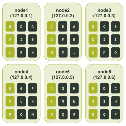
Using this we can see what happens if we had the same outage as the single token cluster did, that is, node3 and node6 are unavailable. As we can see node3 and node6 are both responsible for tokens C, D, I, J, P, and Q. Hence, data associated with those tokens would be unavailable if our application is using a Consistency Level of LOCAL_QUORUM. To put that in different terms, unlike our single token cluster, in this case 33.3% of our data could no longer be retrieved.
Rack ‘em up
A seasoned Cassandra operator will notice that so far we have run our token distribution tests on clusters with only a single rack. To help increase the availability when using vnodes racks can be deployed. When racks are used Cassandra will try to place single replicas in each rack. That is, it will try to ensure no two identical token ranges appear in the same rack.
The key here is to configure the cluster so that for a given datacenter the number of racks is the same as the replication factor.
Let’s retry our previous example where we set num_tokens to 3, only this time we’ll define three racks in the test cluster. After configuring and starting the nodes in ccm, our newly configured test cluster initially looks like this:
$ ccm node1 nodetool status

Datacenter: datacenter1
=======================
Status=Up/Down
|/ State=Normal/Leaving/Joining/Moving
--  Address    Load       Tokens  Owns (effective)  Host ID                               Rack
UN  127.0.0.1  71.08 KiB  3       31.8%             49df615d-bfe5-46ce-a8dd-4748c086f639  rack1
UN  127.0.0.2  71.04 KiB  3       34.4%             3fef187e-00f5-476d-b31f-7aa03e9d813c  rack2
UN  127.0.0.3  66.04 KiB  3       37.3%             c6a0a5f4-91f8-4bd1-b814-1efc3dae208f  rack3
UN  127.0.0.4  109.79 KiB  3      52.9%             74ac0727-c03b-476b-8f52-38c154cfc759  rack1
UN  127.0.0.5  66.09 KiB  3       18.7%             5153bad4-07d7-4a24-8066-0189084bbc80  rack2
UN  127.0.0.6  66.09 KiB  3       25.0%             6693214b-a599-4f58-b1b4-a6cf0dd684ba  rack3
We can still see signs that the cluster might be unbalanced. This is a side issue, as the main point to take from the above is that we now have three racks defined in the cluster with two nodes assigned in each. Once again, similar to the single node cluster, we can create the test keyspace and populate it using cqlsh. We then grab a read out of the token ring to see what it looks like. Same as the previous tests, to make the example easier to follow, we manually add a letter representation next to each token number.
ccm node1 nodetool ring test_keyspace


Datacenter: datacenter1
==========
Address    Rack   Status  State   Load        Owns    Token                 Token Letter
                                                      8993942771016137629   R
127.0.0.5  rack2  Up      Normal  122.42 KiB  34.65%  -8459555739932651620  A
127.0.0.4  rack1  Up      Normal  111.07 KiB  53.84%  -8458588239787937390  B
127.0.0.3  rack3  Up      Normal  116.12 KiB  60.72%  -8347996802899210689  C
127.0.0.1  rack1  Up      Normal  121.31 KiB  46.16%  -5712162437894176338  D
127.0.0.4  rack1  Up      Normal  111.07 KiB  53.84%  -2744262056092270718  E
127.0.0.6  rack3  Up      Normal  122.39 KiB  39.28%  -2132400046698162304  F
127.0.0.2  rack2  Up      Normal  121.42 KiB  65.35%  -1232974565497331829  G
127.0.0.4  rack1  Up      Normal  111.07 KiB  53.84%  1026323925278501795   H
127.0.0.2  rack2  Up      Normal  121.42 KiB  65.35%  3093888090255198737   I
127.0.0.2  rack2  Up      Normal  121.42 KiB  65.35%  3596129656253861692   J
127.0.0.3  rack3  Up      Normal  116.12 KiB  60.72%  3674189467337391158   K
127.0.0.5  rack2  Up      Normal  122.42 KiB  34.65%  3846303495312788195   L
127.0.0.1  rack1  Up      Normal  121.31 KiB  46.16%  4699181476441710984   M
127.0.0.1  rack1  Up      Normal  121.31 KiB  46.16%  6795515568417945696   N
127.0.0.3  rack3  Up      Normal  116.12 KiB  60.72%  7964270297230943708   O
127.0.0.5  rack2  Up      Normal  122.42 KiB  34.65%  8105847793464083809   P
127.0.0.6  rack3  Up      Normal  122.39 KiB  39.28%  8813162133522758143   Q
127.0.0.6  rack3  Up      Normal  122.39 KiB  39.28%  8993942771016137629   R
Once again we capture the output of ccm node1 nodetool describering test_keyspace and change the token numbers to the corresponding letters in the above token ring.
$ ccm node1 nodetool describering test_keyspace

Schema Version:aff03498-f4c1-3be1-b133-25503becf208
TokenRange:
    TokenRange(start_token:B, end_token:C, endpoints:[127.0.0.3, 127.0.0.1, 127.0.0.2], rpc_endpoints:[127.0.0.3, 127.0.0.1, 127.0.0.2], endpoint_details:[EndpointDetails(host:127.0.0.3, datacenter:datacenter1, rack:rack3), EndpointDetails(host:127.0.0.1, datacenter:datacenter1, rack:rack1), EndpointDetails(host:127.0.0.2, datacenter:datacenter1, rack:rack2)])
    TokenRange(start_token:L, end_token:M, endpoints:[127.0.0.1, 127.0.0.3, 127.0.0.5], rpc_endpoints:[127.0.0.1, 127.0.0.3, 127.0.0.5], endpoint_details:[EndpointDetails(host:127.0.0.1, datacenter:datacenter1, rack:rack1), EndpointDetails(host:127.0.0.3, datacenter:datacenter1, rack:rack3), EndpointDetails(host:127.0.0.5, datacenter:datacenter1, rack:rack2)])
    TokenRange(start_token:N, end_token:O, endpoints:[127.0.0.3, 127.0.0.5, 127.0.0.4], rpc_endpoints:[127.0.0.3, 127.0.0.5, 127.0.0.4], endpoint_details:[EndpointDetails(host:127.0.0.3, datacenter:datacenter1, rack:rack3), EndpointDetails(host:127.0.0.5, datacenter:datacenter1, rack:rack2), EndpointDetails(host:127.0.0.4, datacenter:datacenter1, rack:rack1)])
    TokenRange(start_token:P, end_token:Q, endpoints:[127.0.0.6, 127.0.0.5, 127.0.0.4], rpc_endpoints:[127.0.0.6, 127.0.0.5, 127.0.0.4], endpoint_details:[EndpointDetails(host:127.0.0.6, datacenter:datacenter1, rack:rack3), EndpointDetails(host:127.0.0.5, datacenter:datacenter1, rack:rack2), EndpointDetails(host:127.0.0.4, datacenter:datacenter1, rack:rack1)])
    TokenRange(start_token:K, end_token:L, endpoints:[127.0.0.5, 127.0.0.1, 127.0.0.3], rpc_endpoints:[127.0.0.5, 127.0.0.1, 127.0.0.3], endpoint_details:[EndpointDetails(host:127.0.0.5, datacenter:datacenter1, rack:rack2), EndpointDetails(host:127.0.0.1, datacenter:datacenter1, rack:rack1), EndpointDetails(host:127.0.0.3, datacenter:datacenter1, rack:rack3)])
    TokenRange(start_token:R, end_token:A, endpoints:[127.0.0.5, 127.0.0.4, 127.0.0.3], rpc_endpoints:[127.0.0.5, 127.0.0.4, 127.0.0.3], endpoint_details:[EndpointDetails(host:127.0.0.5, datacenter:datacenter1, rack:rack2), EndpointDetails(host:127.0.0.4, datacenter:datacenter1, rack:rack1), EndpointDetails(host:127.0.0.3, datacenter:datacenter1, rack:rack3)])
    TokenRange(start_token:I, end_token:J, endpoints:[127.0.0.2, 127.0.0.3, 127.0.0.1], rpc_endpoints:[127.0.0.2, 127.0.0.3, 127.0.0.1], endpoint_details:[EndpointDetails(host:127.0.0.2, datacenter:datacenter1, rack:rack2), EndpointDetails(host:127.0.0.3, datacenter:datacenter1, rack:rack3), EndpointDetails(host:127.0.0.1, datacenter:datacenter1, rack:rack1)])
    TokenRange(start_token:Q, end_token:R, endpoints:[127.0.0.6, 127.0.0.5, 127.0.0.4], rpc_endpoints:[127.0.0.6, 127.0.0.5, 127.0.0.4], endpoint_details:[EndpointDetails(host:127.0.0.6, datacenter:datacenter1, rack:rack3), EndpointDetails(host:127.0.0.5, datacenter:datacenter1, rack:rack2), EndpointDetails(host:127.0.0.4, datacenter:datacenter1, rack:rack1)])
    TokenRange(start_token:E, end_token:F, endpoints:[127.0.0.6, 127.0.0.2, 127.0.0.4], rpc_endpoints:[127.0.0.6, 127.0.0.2, 127.0.0.4], endpoint_details:[EndpointDetails(host:127.0.0.6, datacenter:datacenter1, rack:rack3), EndpointDetails(host:127.0.0.2, datacenter:datacenter1, rack:rack2), EndpointDetails(host:127.0.0.4, datacenter:datacenter1, rack:rack1)])
    TokenRange(start_token:H, end_token:I, endpoints:[127.0.0.2, 127.0.0.3, 127.0.0.1], rpc_endpoints:[127.0.0.2, 127.0.0.3, 127.0.0.1], endpoint_details:[EndpointDetails(host:127.0.0.2, datacenter:datacenter1, rack:rack2), EndpointDetails(host:127.0.0.3, datacenter:datacenter1, rack:rack3), EndpointDetails(host:127.0.0.1, datacenter:datacenter1, rack:rack1)])
    TokenRange(start_token:D, end_token:E, endpoints:[127.0.0.4, 127.0.0.6, 127.0.0.2], rpc_endpoints:[127.0.0.4, 127.0.0.6, 127.0.0.2], endpoint_details:[EndpointDetails(host:127.0.0.4, datacenter:datacenter1, rack:rack1), EndpointDetails(host:127.0.0.6, datacenter:datacenter1, rack:rack3), EndpointDetails(host:127.0.0.2, datacenter:datacenter1, rack:rack2)])
    TokenRange(start_token:A, end_token:B, endpoints:[127.0.0.4, 127.0.0.3, 127.0.0.2], rpc_endpoints:[127.0.0.4, 127.0.0.3, 127.0.0.2], endpoint_details:[EndpointDetails(host:127.0.0.4, datacenter:datacenter1, rack:rack1), EndpointDetails(host:127.0.0.3, datacenter:datacenter1, rack:rack3), EndpointDetails(host:127.0.0.2, datacenter:datacenter1, rack:rack2)])
    TokenRange(start_token:C, end_token:D, endpoints:[127.0.0.1, 127.0.0.6, 127.0.0.2], rpc_endpoints:[127.0.0.1, 127.0.0.6, 127.0.0.2], endpoint_details:[EndpointDetails(host:127.0.0.1, datacenter:datacenter1, rack:rack1), EndpointDetails(host:127.0.0.6, datacenter:datacenter1, rack:rack3), EndpointDetails(host:127.0.0.2, datacenter:datacenter1, rack:rack2)])
    TokenRange(start_token:F, end_token:G, endpoints:[127.0.0.2, 127.0.0.4, 127.0.0.3], rpc_endpoints:[127.0.0.2, 127.0.0.4, 127.0.0.3], endpoint_details:[EndpointDetails(host:127.0.0.2, datacenter:datacenter1, rack:rack2), EndpointDetails(host:127.0.0.4, datacenter:datacenter1, rack:rack1), EndpointDetails(host:127.0.0.3, datacenter:datacenter1, rack:rack3)])
    TokenRange(start_token:O, end_token:P, endpoints:[127.0.0.5, 127.0.0.6, 127.0.0.4], rpc_endpoints:[127.0.0.5, 127.0.0.6, 127.0.0.4], endpoint_details:[EndpointDetails(host:127.0.0.5, datacenter:datacenter1, rack:rack2), EndpointDetails(host:127.0.0.6, datacenter:datacenter1, rack:rack3), EndpointDetails(host:127.0.0.4, datacenter:datacenter1, rack:rack1)])
    TokenRange(start_token:J, end_token:K, endpoints:[127.0.0.3, 127.0.0.5, 127.0.0.1], rpc_endpoints:[127.0.0.3, 127.0.0.5, 127.0.0.1], endpoint_details:[EndpointDetails(host:127.0.0.3, datacenter:datacenter1, rack:rack3), EndpointDetails(host:127.0.0.5, datacenter:datacenter1, rack:rack2), EndpointDetails(host:127.0.0.1, datacenter:datacenter1, rack:rack1)])
    TokenRange(start_token:G, end_token:H, endpoints:[127.0.0.4, 127.0.0.2, 127.0.0.3], rpc_endpoints:[127.0.0.4, 127.0.0.2, 127.0.0.3], endpoint_details:[EndpointDetails(host:127.0.0.4, datacenter:datacenter1, rack:rack1), EndpointDetails(host:127.0.0.2, datacenter:datacenter1, rack:rack2), EndpointDetails(host:127.0.0.3, datacenter:datacenter1, rack:rack3)])
    TokenRange(start_token:M, end_token:N, endpoints:[127.0.0.1, 127.0.0.3, 127.0.0.5], rpc_endpoints:[127.0.0.1, 127.0.0.3, 127.0.0.5], endpoint_details:[EndpointDetails(host:127.0.0.1, datacenter:datacenter1, rack:rack1), EndpointDetails(host:127.0.0.3, datacenter:datacenter1, rack:rack3), EndpointDetails(host:127.0.0.5, datacenter:datacenter1, rack:rack2)])
Lastly, we once again determine all the token ranges assigned to each node:
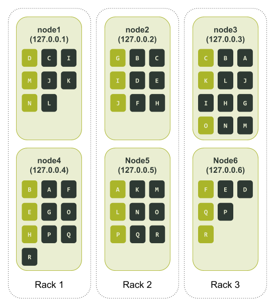
As we can see from the way Cassandra has assigned the tokens, there is now a complete data replica spread across two nodes in each of our three racks. If we go back to our failure scenario where node3 and node6 become unavailable, we can still service queries using a Consistency Level of LOCAL_QUORUM. The only elephant in the room here is node3 has a lot more tokens distributed to it than other nodes. Its counterpart in the same rack, node6, is at the opposite end with fewer tokens allocated to it.
Too many vnodes spoil the cluster
Given the token distribution issues with a low numbers of vnodes, one would think the best option is to have a large vnode value. However, apart from having a higher chance of some data being unavailable in a multi-node outage, large vnode values also impact streaming operations. To repair data on a node, Cassandra will start one repair session per vnode. These repair sessions need to be processed sequentially. Hence, the larger the vnode value the longer the repair times, and the overhead needed to run a repair.
In an effort to fix slow repair times as a result of large vnode values, CASSANDRA-5220 was introduced in 3.0. This change allows Cassandra to group common token ranges for a set of nodes into a single repair session. It increased the size of the repair session as multiple token ranges were being repaired, but reduced the number of repair sessions being executed in parallel.
We can see the effect that vnodes have on repair by running a simple test on a cluster backed by real hardware. To do this test we first need create a cluster that uses single tokens run a repair. Then we can create the same cluster except with 256 vnodes, and run the same repair. We will use tlp-cluster to create a Cassandra cluster in AWS with the following properties.
- Instance size: i3.2xlarge
- Node count: 12
- Rack count: 3 (4 nodes per rack)
- Cassandra version: 3.11.9 (latest stable release at the time of writing)
The commands to build this cluster are as follows.
$ tlp-cluster init --azs a,b,c --cassandra 12 --instance i3.2xlarge --stress 1 TLP BLOG "Blogpost repair testing"
$ tlp-cluster up
$ tlp-cluster use --config "cluster_name:SingleToken" --config "num_tokens:1" 3.11.9
$ tlp-cluster install
Once we provision the hardware we set the initial_token property for each of the nodes individually. We can calculate the initial tokens for each node using a simple Python command.
Python 2.7.16 (default, Nov 23 2020, 08:01:20)
[GCC Apple LLVM 12.0.0 (clang-1200.0.30.4) [+internal-os, ptrauth-isa=sign+stri on darwin
Type "help", "copyright", "credits" or "license" for more information.
>>> num_tokens = 1
>>> num_nodes = 12
>>> print("\n".join(['[Node {}] initial_token: {}'.format(n + 1, ','.join([str(((2**64 / (num_tokens * num_nodes)) * (t * num_nodes + n)) - 2**63) for t in range(num_tokens)])) for n in range(num_nodes)]))
[Node 1] initial_token: -9223372036854775808
[Node 2] initial_token: -7686143364045646507
[Node 3] initial_token: -6148914691236517206
[Node 4] initial_token: -4611686018427387905
[Node 5] initial_token: -3074457345618258604
[Node 6] initial_token: -1537228672809129303
[Node 7] initial_token: -2
[Node 8] initial_token: 1537228672809129299
[Node 9] initial_token: 3074457345618258600
[Node 10] initial_token: 4611686018427387901
[Node 11] initial_token: 6148914691236517202
[Node 12] initial_token: 7686143364045646503
After starting Cassandra on all the nodes, around 3 GB of data per node can be preloaded using the following tlp-stress command. In this command we set our keyspace replication factor to 3 and set gc_grace_seconds to 0. This is done to make hints expire immediately when they are created, which ensures they are never delivered to the destination node.
ubuntu@ip-172-31-19-180:~$ tlp-stress run KeyValue --replication "{'class': 'NetworkTopologyStrategy', 'us-west-2':3 }" --cql "ALTER TABLE tlp_stress.keyvalue WITH gc_grace_seconds = 0" --reads 1 --partitions 100M --populate 100M --iterations 1
Upon completion of the data loading, the cluster status looks like this.
ubuntu@ip-172-31-30-95:~$ nodetool status
Datacenter: us-west-2
=====================
Status=Up/Down
|/ State=Normal/Leaving/Joining/Moving
--  Address        Load       Tokens       Owns (effective)  Host ID                               Rack
UN  172.31.30.95   2.78 GiB   1            25.0%             6640c7b9-c026-4496-9001-9d79bea7e8e5  2a
UN  172.31.31.106  2.79 GiB   1            25.0%             ceaf9d56-3a62-40be-bfeb-79a7f7ade402  2a
UN  172.31.2.74    2.78 GiB   1            25.0%             4a90b071-830e-4dfe-9d9d-ab4674be3507  2c
UN  172.31.39.56   2.79 GiB   1            25.0%             37fd3fe0-598b-428f-a84b-c27fc65ee7d5  2b
UN  172.31.31.184  2.78 GiB   1            25.0%             40b4e538-476a-4f20-a012-022b10f257e9  2a
UN  172.31.10.87   2.79 GiB   1            25.0%             fdccabef-53a9-475b-9131-b73c9f08a180  2c
UN  172.31.18.118  2.79 GiB   1            25.0%             b41ab8fe-45e7-4628-94f0-a4ec3d21f8d0  2a
UN  172.31.35.4    2.79 GiB   1            25.0%             246bf6d8-8deb-42fe-bd11-05cca8f880d7  2b
UN  172.31.40.147  2.79 GiB   1            25.0%             bdd3dd61-bb6a-4849-a7a6-b60a2b8499f6  2b
UN  172.31.13.226  2.79 GiB   1            25.0%             d0389979-c38f-41e5-9836-5a7539b3d757  2c
UN  172.31.5.192   2.79 GiB   1            25.0%             b0031ef9-de9f-4044-a530-ffc67288ebb6  2c
UN  172.31.33.0    2.79 GiB   1            25.0%             da612776-4018-4cb7-afd5-79758a7b9cf8  2b
We can then run a full repair on each node using the following commands.
$ source env.sh
$ c_all "nodetool repair -full tlp_stress"
The repair times recorded for each node were.
[2021-01-22 20:20:13,952] Repair command #1 finished in 3 minutes 55 seconds
[2021-01-22 20:23:57,053] Repair command #1 finished in 3 minutes 36 seconds
[2021-01-22 20:27:42,123] Repair command #1 finished in 3 minutes 32 seconds
[2021-01-22 20:30:57,654] Repair command #1 finished in 3 minutes 21 seconds
[2021-01-22 20:34:27,740] Repair command #1 finished in 3 minutes 17 seconds
[2021-01-22 20:37:40,449] Repair command #1 finished in 3 minutes 23 seconds
[2021-01-22 20:41:32,391] Repair command #1 finished in 3 minutes 36 seconds
[2021-01-22 20:44:52,917] Repair command #1 finished in 3 minutes 25 seconds
[2021-01-22 20:47:57,729] Repair command #1 finished in 2 minutes 58 seconds
[2021-01-22 20:49:58,868] Repair command #1 finished in 1 minute 58 seconds
[2021-01-22 20:51:58,724] Repair command #1 finished in 1 minute 53 seconds
[2021-01-22 20:54:01,100] Repair command #1 finished in 1 minute 50 seconds
These times give us a total repair time of 36 minutes and 44 seconds.
The same cluster can be reused to test repair times when 256 vnodes are used. To do this we execute the following steps.
- Shut down Cassandra on all the nodes.
- Delete the contents in each of the directories
data,commitlog,hints, andsaved_caches(these are located in /var/lib/cassandra/ on each node). - Set
num_tokensin the cassandra.yaml configuration file to a value of 256 and remove theinitial_tokensetting. - Start up Cassandra on all the nodes.
After populating the cluster with data its status looked like this.
ubuntu@ip-172-31-30-95:~$ nodetool status
Datacenter: us-west-2
=====================
Status=Up/Down
|/ State=Normal/Leaving/Joining/Moving
--  Address        Load       Tokens       Owns (effective)  Host ID                               Rack
UN  172.31.30.95   2.79 GiB   256          24.3%             10b0a8b5-aaa6-4528-9d14-65887a9b0b9c  2a
UN  172.31.2.74    2.81 GiB   256          24.4%             a748964d-0460-4f86-907d-a78edae2a2cb  2c
UN  172.31.31.106  3.1 GiB    256          26.4%             1fc68fbd-335d-4689-83b9-d62cca25c88a  2a
UN  172.31.31.184  2.78 GiB   256          23.9%             8a1b25e7-d2d8-4471-aa76-941c2556cc30  2a
UN  172.31.39.56   2.73 GiB   256          23.5%             3642a964-5d21-44f9-b330-74c03e017943  2b
UN  172.31.10.87   2.95 GiB   256          25.4%             540a38f5-ad05-4636-8768-241d85d88107  2c
UN  172.31.18.118  2.99 GiB   256          25.4%             41b9f16e-6e71-4631-9794-9321a6e875bd  2a
UN  172.31.35.4    2.96 GiB   256          25.6%             7f62d7fd-b9c2-46cf-89a1-83155feebb70  2b
UN  172.31.40.147  3.26 GiB   256          27.4%             e17fd867-2221-4fb5-99ec-5b33981a05ef  2b
UN  172.31.13.226  2.91 GiB   256          25.0%             4ef69969-d9fe-4336-9618-359877c4b570  2c
UN  172.31.33.0    2.74 GiB   256          23.6%             298ab053-0c29-44ab-8a0a-8dde03b4f125  2b
UN  172.31.5.192   2.93 GiB   256          25.2%             7c690640-24df-4345-aef3-dacd6643d6c0  2c
When we run the same repair test for the single token cluster on the vnode cluster, the following repair times were recorded.
[2021-01-22 22:45:56,689] Repair command #1 finished in 4 minutes 40 seconds
[2021-01-22 22:50:09,170] Repair command #1 finished in 4 minutes 6 seconds
[2021-01-22 22:54:04,820] Repair command #1 finished in 3 minutes 43 seconds
[2021-01-22 22:57:26,193] Repair command #1 finished in 3 minutes 27 seconds
[2021-01-22 23:01:23,554] Repair command #1 finished in 3 minutes 44 seconds
[2021-01-22 23:04:40,523] Repair command #1 finished in 3 minutes 27 seconds
[2021-01-22 23:08:20,231] Repair command #1 finished in 3 minutes 23 seconds
[2021-01-22 23:11:01,230] Repair command #1 finished in 2 minutes 45 seconds
[2021-01-22 23:13:48,682] Repair command #1 finished in 2 minutes 40 seconds
[2021-01-22 23:16:23,630] Repair command #1 finished in 2 minutes 32 seconds
[2021-01-22 23:18:56,786] Repair command #1 finished in 2 minutes 26 seconds
[2021-01-22 23:21:38,961] Repair command #1 finished in 2 minutes 30 seconds
These times give us a total repair time of 39 minutes and 23 seconds.
While the time difference is quite small for 3 GB of data per node (up to an additional 45 seconds per node), it is easy to see how the difference could balloon out when we have data sizes in the order of hundreds of gigabytes per node.
Unfortunately, all data streaming operations like bootstrap and datacenter rebuild fall victim to the same issue repairs have with large vnode values. Specifically, when a node needs to stream data to another node a streaming session is opened for each token range on the node. This results in a lot of unnecessary overhead, as data is transferred via the JVM.
Secondary indexes impacted too
To add insult to injury, the negative effect of a large vnode values extends to secondary indexes because of the way the read path works.
When a coordinator node receives a secondary index request from a client, it fans out the request to all the nodes in the cluster or datacenter depending on the locality of the consistency level. Each node then checks the SSTables for each of the token ranges assigned to it for a match to the secondary index query. Matches to the query are then returned to the coordinator node.
Hence, the larger the number of vnodes, the larger the impact to the responsiveness of the secondary index query. Furthermore, the performance impacts on secondary indexes grow exponentially with the number of replicas in the cluster. In a scenario where multiple datacenters have nodes using many vnodes, secondary indexes become even more inefficient.
A new hope
So what we are left with then is a property in Cassandra that really hits the mark in terms of reducing the complexities when resizing a cluster. Unfortunately, their benefits come at the expense of unbalanced token ranges on one end, and degraded operations performance at the other. That being said, the vnodes story is far from over.
Eventually, it became a well-known fact in the Apache Cassandra project that large vnode values had undesirable side effects on a cluster. To combat this issue, clever contributors and committers added CASSANDRA-7032 in 3.0; a replica aware token allocation algorithm. The idea was to allow a low value to be used for num_tokens while maintaining relatively even balanced token ranges. The enhancement includes the addition of the allocate_tokens_for_keyspace setting in the cassandra.yaml file. The new algorithm is used instead of the random token allocator when an existing user keyspace is assigned to the allocate_tokens_for_keyspace setting.
Behind the scenes, Cassandra takes the replication factor of the defined keyspace and uses it when calculating the token values for the node when it first enters the cluster. Unlike the random token generator, the replica aware generator is like an experienced member of a symphony orchestra; sophisticated and in tune with its surroundings. So much so, that the process it uses to generate token ranges involves:
- Constructing an initial token ring state.
- Computing candidates for new tokens by splitting all existing token ranges right in the middle.
- Evaluating the expected improvements from all candidates and forming a priority queue.
- Iterating through the candidates in the queue and selecting the best combination.
- During token selection, re-evaluate the candidate improvements in the queue.
While this was good advancement for Cassandra, there are a few gotchas to watch out for when using the replica aware token allocation algorithm. To start with, it only works with the Murmur3Partitioner partitioner. If you started with an old cluster that used another partitioner such as the RandomPartitioner and have upgraded over time to 3.0, the feature is unusable. The second and more common stumbling block is that some trickery is required to use this feature when creating a cluster from scratch. The question was common enough that we wrote a blog post specifically on how to use the new replica aware token allocation algorithm to set up a new cluster with even token distribution.
As you can see, Cassandra 3.0 made a genuine effort to address vnode’s rough edges. What’s more, there are additional beacons of light on the horizon with the upcoming Cassandra 4.0 major release. For instance, a new allocate_tokens_for_local_replication_factor setting has been added to the cassandra.yaml file via CASSANDRA-15260. Similar to its cousin the allocate_tokens_for_keyspace setting, the replica aware token allocation algorithm is activated when a value is supplied to it.
However, unlike its close relative, it is more user-friendly. This is because no phaffing is required to create a balanced cluster from scratch. In the simplest case, you can set a value for the allocate_tokens_for_local_replication_factor setting and just start adding nodes. Advanced operators can still manually assign tokens to the initial nodes to ensure the desired replication factor is met. After that, subsequent nodes can be added with the replication factor value assigned to the allocate_tokens_for_local_replication_factor setting.
Arguably, one of the longest time coming and significant changes to be released with Cassandra 4.0 is the update to the default value of the num_tokens setting. As mentioned at the beginning of this post thanks to CASSANDRA-13701 Cassandra 4.0 will ship with a num_tokens value set to 16 in the cassandra.yaml file. In addition, the allocate_tokens_for_local_replication_factor setting is enabled by default and set to a value of 3.
These changes are much better user defaults. On a vanilla installation of Cassandra 4.0, the replica aware token allocation algorithm kicks in as soon as there are enough hosts to satisfy a replication factor of 3. The result is an evenly distributed token ranges for new nodes with all the benefits that a low vnodes value has to offer.
Conclusion
The consistent hashing and token allocation functionality form part of Cassandra’s backbone. Virtual nodes take the guess work out of maintaining this critical functionality, specifically, making cluster resizing quicker and easier. As a rule of thumb, the lower the number of vnodes, the less even the token distribution will be, leading to some nodes being over worked. Alternatively, the higher the number of vnodes, the slower cluster wide operations take to complete and more likely data will be unavailable if multiple nodes are down. The features in 3.0 and the enhancements to those features thanks to 4.0, allow Cassandra to use a low number of vnodes while still maintaining a relatively even token distribution. Ultimately, it will produce a better out-of-the-box experience for new users when running a vanilla installation of Cassandra 4.0.