This is our third post in our series on performance tuning with Apache Cassandra. In our first post, we discussed how we can use Flame Graphs to visually diagnose performance problems. In our second post, we discussed JVM tuning, and how the different JVM settings can have an affect on different workloads.

In this post, we’ll dig into a table level setting which is usually overlooked: compression. Compression options can be specified when creating or altering a table, and it defaults to enabled if not specified. The default is great when working with write heavy workloads, but can become a problem on read heavy and mixed workloads.

Before we get into optimizations, let’s take a step back to understand the basics of compression in Cassandra. Once we’ve built a foundation of knowledge, we’ll see how to apply it to real world workloads.

How it works

When we create a table in Cassandra, we can specify a variety of table options in addition to our fields. In addition to options such as using TWCS for our compaction strategy, specifying gc grace seconds, and caching options, we can also tell Cassandra how we want it to compress our data. If the compression option is not specified, LZ4Compressor will be used, which is known for it’s excellent performance and compression rate. In addition to the algorithm, we can specify our chunk_length_in_kb, which is the size of the uncompressed buffer we write our data to as an intermediate step before writing to disk. Here’s an example of a table using LZ4Compressor with 64KB chunk length:

create table sensor_data ( 
    id text primary key, 
    data text) 
WITH compression = {'sstable_compression': 'LZ4Compressor', 
                    'chunk_length_kb': 64};

We can examine how well compression is working at the table level by checking tablestats:

$ bin/nodetool tablestats tlp_stress

Keyspace : tlp_stress
	Read Count: 89766
	Read Latency: 0.18743983245326737 ms
	Write Count: 8880859
	Write Latency: 0.009023213069816781 ms
	Pending Flushes: 0
		Table: sensor_data
		SSTable count: 5
		Old SSTable count: 0
		Space used (live): 864131294
		Space used (total): 864131294
		Off heap memory used (total): 2472433
		SSTable Compression Ratio: 0.8964684393508305
		Compression metadata off heap memory used: 140544

The SSTable Compression Ratio line above tells us how effective compression is. Compression ratio is calculated by the following:

compressionRatio = (double) compressed/uncompressed;

meaning the smaller the number, the better the compression. In the above example our compressed data is taking up almost 90% of the original data, which isn’t particularly great.

How data is written

I’ve found digging into the codebase, profiling and working with a debugger to be the most effective way to learn how software works.

When data is written to / read from SSTables, we’re not dealing with convenient typed objects, we’re dealing with streams of bytes. Our compressed data is written in the CompressedSequentialWriter class, which extends BufferedDataOutputStreamPlus. This writer uses a temporary buffer. When the data is written out to disk the buffer is compressed and some meta data about it is recorded to a CompressionInfo file. If there is more data than available space in the buffer, the buffer is written to, flushed, and the buffer starts fresh to be written to again (and perhaps flushed again). You can see this in org/apache/cassandra/io/util/BufferedDataOutputStreamPlus.java:

@Override
public void write(byte[] b, int off, int len) throws IOException
{
    if (b == null)
        throw new NullPointerException();

    // avoid int overflow
    if (off < 0 || off > b.length || len < 0
        || len > b.length - off)
        throw new IndexOutOfBoundsException();

    if (len == 0)
        return;

    int copied = 0;
    while (copied < len)
    {
        if (buffer.hasRemaining())
        {
            int toCopy = Math.min(len - copied, buffer.remaining());
            buffer.put(b, off + copied, toCopy);
            copied += toCopy;
        }
        else
        {
            doFlush(len - copied);
        }
    }
}

The size of this buffer is determined by chunk_length_in_kb.

How data is read

The read path in Cassandra is (more or less) the opposite of the write path. We pull chunks out of SSTables, decompress them, and return them to the client. The full path is a little more complex - there’s a a ChunkCache (managed by caffeine) that we go through, but that’s beyond the scope of this post.

During the read path, the entire chunk must be read and decompressed. We’re not able to selectively read only the bytes we need. The impact of this is that if we are using 4K chunks, we can get away with only reading 4K off disk. If we use 256KB chunks, we have to read the entire 256K. This might be fine for a handful of requests but when trying to maximize throughput we need to consider what happens when we have requests in the thousands per second. If we have to read 256KB off disk for ten thousand requests a second, we’re going to need to read 2.5GB per second off disk, and that can be an issue no matter what hardware we are using.

What about page cache?

Linux will automatically leverage any RAM that’s not being used by applications to keep recently accessed filesystem blocks in memory. We can see how much page cache we’re using by using the free tool:

$ free -mhw
              total        used        free      shared     buffers       cache   available
Mem:            62G        823M         48G        1.7M        261M         13G         61G
Swap:          8.0G          0B        8.0G

Page cache can be a massive benefit if you have a working data set that fits in memory. With smaller data sets this is incredibly useful, but Cassandra was built to solve big data problems. Typically that means having a lot more data than available RAM. If our working data set on each node is 2 TB, and we only have 20-30 GB of free RAM, it’s very possible we’ll serve almost none of our requests out of cache. Yikes.

Ultimately, we need to ensure we use a chunk length that allows us to minimize our I/O. Larger chunks can compress better, giving us a smaller disk footprint, but we end up needing more hardware, so the space savings becomes meaningless for certain workloads. There’s no perfect setting that we can apply to every workload. Frequently, the most reads you do, the smaller the chunk size. Even this doesn’t apply uniformly; larger requests will hit more chunks, and will benefit from a larger chunk size.

The Benchmarks

Alright - enough with the details! We’re going to run a simple benchmark to test how Cassandra performs with a mix of read and write requets with a simple key value data model. We’ll be doing this using our stress tool, tlp-stress (commit 40cb2d28fde). We will get into the details of this stress tool in a later post - for now all we need to cover is that it includes a key value workload out of the box we can leverage here.

For this test I installed Apache Cassandra 3.11.3 on an AWS c5d.4xlarge instance running Ubuntu 16.04 following the instructions on cassandra.apache.org, and updated all the system packages using apt-get upgrade. I’m only using a single node here in order to isolate the compression settings and not introduce noise from the network overhead of running a full cluster.

The ephemeral NVMe disk is using XFS and mounted it at /var/lib/cassandra. I set readahead using blockdev --setra 0 /dev/nvme1n1 so we can see the impact that compression has on our disk requests and not hide it with page cache.

For each workload, I put the following command in a shell script, and ran tlp-stress from a separate c5d.4xlarge instance (passing the chunk size as the first parameter):

$ bin/tlp-stress run KeyValue -i 10B -p 10M --populate -t 4 \
  --replication "{'class':'SimpleStrategy', 'replication_factor':1}" \
  --field.keyvalue.value='book(100,200)' -r .5  \
  --compression "{'chunk_length_in_kb': '$1', 'class': 'org.apache.cassandra.io.compress.LZ4Compressor'}" \
  --host 172.31.42.30

This runs a key value workload across 10 million partitions (-p 10M), pre-populating the data (--populate), with 50% reads (-r .5), picking 100-200 words from of one of the books included in the stress tool (--field.keyvalue.value='book(100,200)'). We can specify a compression strategy using --compression.

For the test I’ve used slightly modified Cassandra configuration files to reduce the effect of GC pauses by increasing the total heap (12GB) as well as the new gen (6GB). I spend a small amount of time on this as optimizing it perfectly isn’t necessary. I also set compaction throughput to 160.

For the test, I monitored the JVM’s allocate rate using the Swiss Java Knife (sjk-plus) and disk / network / cpu usage with dstat.

Default 64KB Chunk Size

The first test used the default of 64KB chunk length. I started the stress command and walked away to play with my dog for a bit. When I came back, I was through about 35 million requests:

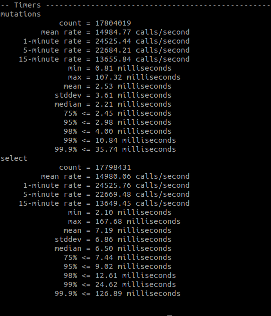
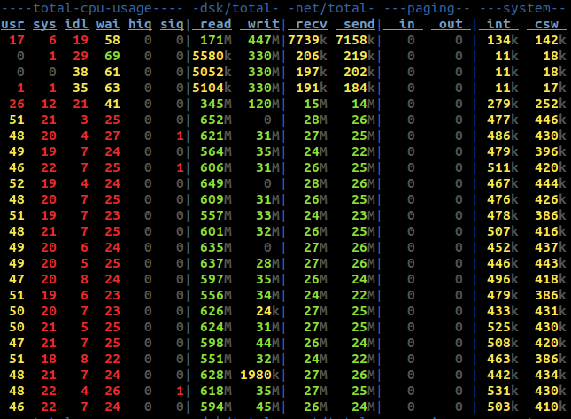
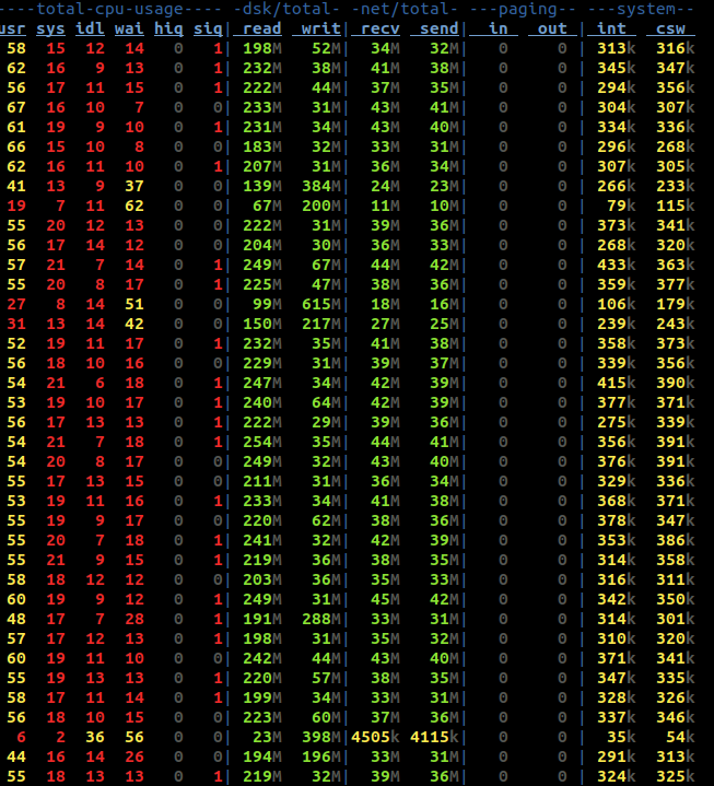
You can see in the above screenshot our 5 minute rate is about 22K writes / second and 22K reads/ second. Looking at the output of dstat at this time, we can see we’re doing between 500 and 600MB / second of reads / second:

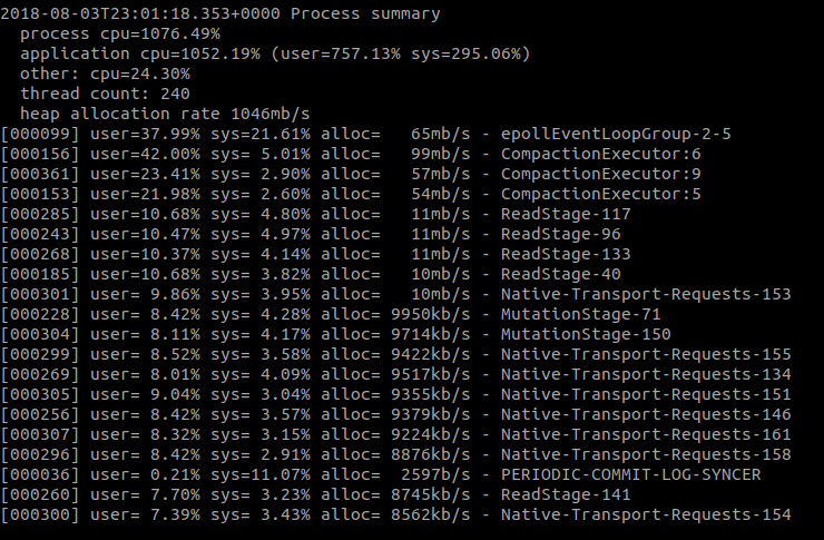
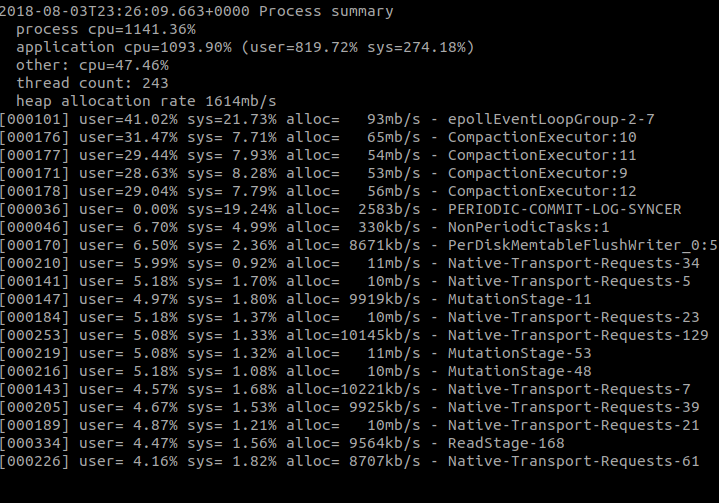
Memory allocation fluctuated a bit, but it hovered around 1GB/s:

Not the most amazing results in the world. Of the disk reads, some of that throughput can be attributed to compaction, which we’ll always have to contend with in the real world. That’s capped at 160MB/s, leaving around 400MB/s to handle reads. That’s a lot considering we’re only sending 25MB across the network. That means we’re doing over 15x the disk I/O than our network I/O. We are very much disk bound in this workload.

4KB Chunk Size

Let’s see if the 4KB chunk size does any better. Before the test I shut down Cassandra, cleared the data directory, and started things back up. I ran the same stress test above using the above shell script, passing 4 as the chunk size. I once again played fetch with my dog for a bit and came back after around the same time as the previous test.

Looking at the stress output, it’s immediately obvious there’s a significant improvement:

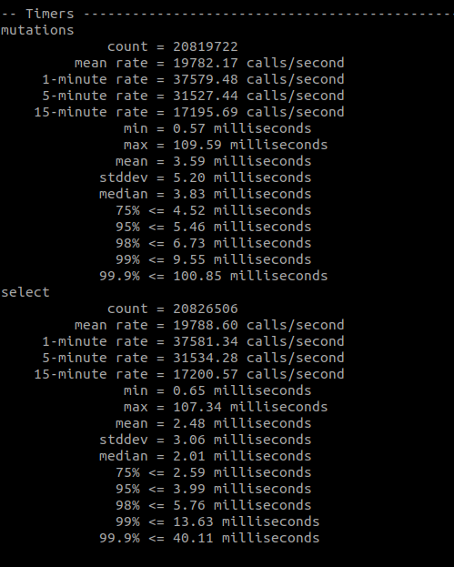
In almost every single metric reported by the metric library the test with 4KB outperforms the 64KB test. Our throughput is better (62K ops / second vs 44K ops / second in the 1 minute rate), and our p99 for reads is better (13ms vs 24ms).

If we’re doing less I/O on each request, how does that impact our total disk and network I/O?

As you can see above, there’s a massive improvement. Disk I/O is significantly reduced from making smaller (but more) requests to disk, and our network I/O is significantly higher from responding to more requests.

It was initially a small surprise to see an increased heap allocation rate (because we’re reading WAY less data into memory), but this is simply the result of doing a lot more requests. There are a lot of objects created in order to satisfy a request; far more than the number created to read the data off disk. More requests results in higher allocation. We’d want to ensure those objects don’t make it into the Old Gen as we go through JVM tuning.

Off Heap Memory Usage

The final thing to consider here is off heap memory usage. Along side each compressed SSTable is compression metadata. The compression files have names like na-9-big-CompressionInfo.db. The compression metadata is stored in memory, off the Cassandra heap. The size of the offheap usage is directly proportional to the amount of chunks used. More chunks = more space used. More chunks are used when a smaller chunk size is used, hence more offheap memory is used to store the metadata for each chunk. It’s important to understand this trade off. A table using 4KB chunks will use 16 times the memory as one using 64KB chunks.

In the example I used above the memory usage can be seen as follows:

Compression metadata off heap memory used: 140544 

Changing Existing Tables

Now that you can see how a smaller chunk size can benefit read heavy and mixed workloads, it’s time to try it out. If you have a table you’d like to change the compression setting on, you can do the following at the cqlsh shell:

cqlsh:tlp_stress> alter table keyvalue with compression = {'sstable_compression': 'LZ4Compressor', 'chunk_length_kb': 4};

New SSTables that are written after this change is applied will use this setting, but existing SSTables won’t be rewritten automatically. Because of this, you shouldn’t expect an immediate performance difference after applying this setting. If you want to rewrite every SSTable immediately, you’ll need to do the following:

nodetool upgradesstables -a tlp_stress keyvalue

Conclusion

The above is a single test demonstrating how a tuning compression settings can affect Cassandra performance in a significant way. Using out of the box settings for compression on read heavy or mixed workloads will almost certainly put unnecessary strain on your disk while hurting your read performance. I highly recommend taking the time to understand your workload and analyze your system resources to understand where your bottleneck is, as there is no absolute correct setting to use for every workload.

Keep in mind the tradeoff between memory and chunk size as well. When working with a memory constrained environment it may seem tempting to use 4KB chunks everywhere, but it’s important to understand that it’ll use more memory. In these cases, it’s a good idea to start with smaller tables that are read from the most.